Random Work - nuwen.net
You load sixteen tons, what do you get?
Contents
This is a collection of interesting things I've examined here and there, or maybe just descriptions of stuff I've learned about. Some is taken from Caltech courses I've been in, and some is independent. Therefore, if you're a Techer, you are bound by the Honor Code not to read solutions for problems that may appear in courses you're taking. Each heading denotes a different chunk of work and a disclaimer will appear underneath ones related to specific courses. Non-Techers can just ignore all of that and get to the good stuff.
All code appearing on this page is mine, and distributed under the GNU GPL.
Ternary sequences
(This was initially written directed at CS1 students, unrelated to any course work.)
I recently read an issue of American Scientist with a cool article about ternary numbers. Here's a description of something in it that interested me, along with some Scheme code for playing around with sequences of ternary numbers.
Let's look at sequences of digits in certain bases. For example, in base 10 one could be 0 1 2 3 4 5 6 7 8 9. (Which I will write as 0123456789 to save space - we won't work with base 11 or higher. :->) We'll call a "square" sequence one that has at least one pair of adjacent identical subsequences. Meaning that it looks like:
[beginning of sequence].....[some subsequence of any length][same subsequence]....[end of sequence].
In base 10, here is a square sequence:
012349879874321
Because:
01234[987][987]4321
We'll call a squarefree sequence one which is not square. Here is a squarefree sequence in base 10:
0123498701234
There are indeed two subsequences [01234] there, and they are identical subsequences - but they are not adjacent.
Now, let's look at base 2 squarefree sequences. How long can they be?
Length one: The sequences 0 and 1 are both squarefree (trivial).
Length two: The sequences 01 and 10 are squarefree; 00 and 11 are not.
Length three: 010 and 101 are squarefree, but 000, 001, 011, 100, 110, and 111 are not squarefree (as they contain either
[0][0] or [1][1]).
Length four: Let's look at all of them:
0000 through 0011 - start with [0][0]
0100 - ends in [0][0]
0101 - is [01][01]
0110 - has [1][1] in the middle
0111 - has [1][1]
1000 - has [0][0]
1001 - has [0][0] in the middle
1010 - is [10][10]
1011 - ends in [1][1]
1100 - 1111 - start with [1][1]
So there are NO squarefree sequences of length four in base 2! (There aren't any of length 5 or higher, either; any
sequence of length 5 must contain as a subsequence one of those sixteen sequences of length 4, and none of those are
squarefree, so the whole length 5 sequence can't be squarefree.)
What about base 3? You might go trying to build a sequence, digit by digit, but then you could get stuck:
0, 01, 010, 0102, 01020, 010201, and 0102010 are all okay. But can we add another digit?
01020100 - ends in [0][0]. Bleah.
01020101 - ends in [01][01]. Bleah.
01020102 - is [0102][0102]. Uh oh.
That is sort of depressing.
However, it turns out that you don't necessarily HAVE to get stuck! The Norwegian mathematican Axel Thue proved nearly 100
years ago that there do exist arbitrarily long ternary squarefree sequences, and gave a method for constructing one. It's simple:
You start with the sequence 0.
To generate the next sequence, perform the following replacements simultaneously:
0 is replaced by 1 2
1 is replaced by 1 0 2
2 is replaced by 0
(So if you were performing this on the sequence 1 0 2 0, you'd get 102 12 0 12. See? Simple.)
Thue proved that you can perform this procedure as many times over as you like, starting with the sequence 0, and you will
always generate a (longer) ternary sequence which is squarefree.
We'll leave the proof of that to mathematics majors, or - better yet - someone who knows how to use a library! We can just implement this in Scheme and see what happens, because having a computer generate these Thue sequences is way easier and faster for us.
First, we need a way to find what subsequence of numbers have to be substituted in, given either 0, 1, or 2. This is an easy function:
(define (thue-lists n)
  (cond ((= n 0) (list 1 2))
        ((= n 1) (list 1 0 2))
        ((= n 2) (list 0))))
Examples:
(thue-lists 0) => (1 2)
(thue-lists 1) => (1 0 2)
(thue-lists 2) => (0)
Now, we want some way to take a list - any list of ternary numbers - and perform the Thue replacement on them.
(define (thue-replace lst) (apply append (map thue-lists lst)))
This replaces every element e in lst with (thue-lists e). (map thue-lists (list 0 1 2 1)) produces ((1 2) (1 0 2) (0) (1 0 2)). apply append then concatenates all of the sublists together, producing (1 2 1 0 2 0 1 0 2).
And finally, we don't want to have to type
(thue-replace (thue-replace (thue-replace (list 0))))
to get the third list in this sequence, so let's make a quick wrapper function:
(define (thue-iterate n)
  (if (= n 0)
      (list 0)
      (thue-replace (thue-iterate (- n 1)))))
Now, (thue-iterate 0) gives us (0). (thue-iterate 1) gives us (1 2). (thue-iterate 2) gives (1 0 2 0).
The fifth Thue sequence is (1 0 2 1 2 0 1 0 2 0 1 2 1 0 2 1 2 0 1 2 1 0 2 0 1 0 2 1 2 0 1 2).
Now, you can check by hand that that is squarefree, or - better yet - we can have a computer do it!
Growth of Thue sequences
(I originally wrote this as an addendum to the above work with Thue sequences, and again it is unrelated to CS1 work.)
I was investigating how (length (thue-iterate n)) grows as n grows. To my astonishment it proceeds 1, 2, 4, 8, 16, 32, 64.... Wowsa!
Ever wary of the Strong Law of Small Numbers (namely, that patterns don't always go as the first cases might indicate), I decided to see if this was, in fact, true.
(For an example of the Strong Law, draw a circle. Arrange dots on the circumference such that when straight lines between every pair of dots are drawn, the circle is divided into the most number of distinct regions with nonzero area. Two dots produce two regions. Three dots produce 4 regions. 4 dots produce 8 regions. But the pattern DOES NOT HOLD!)
The reason this surprised me so much is that another "replacement sequence" which I knew of before grows in a much more nasty fashion:
In which you start with 13. Say it out loud: one one, then one three. Giving 1113. Which is: three ones, one three. Giving 3113. Which is: one three, two ones, one three. Giving 132113. And so forth. It turns out that the manner in which its length grows isn't very nice to compute.
Anyways, back to the "Thue sequences": The proof that its length grows as powers of two is rather nice. Let's do some induction. (Heh).
Now, say that our expression has A number of 0s, B number of 1s, and C number of 2s. The "0 replacement rule" will create A 1s and A 2s in the next expression. The "1 replacement rule" will create B 1s, B 0s, and B 2s in the next expression. And the "2 replacement rule" will create C 0s in the next expression. So, the next expression generated will have: B + C 0s, A + B 1s, and A + B 2s.
Say our expression starts off with N 0s, N-1 1s, and N-1 2s. That sums to 3N-2, the length of the sequence. As noted above, the next sequence will have 2N-2 0s, 2N-1 1s, and 2N-1 2s. That sums to 6N-4, so the length has doubled.
Now, a sequence with 2N-2 0s, 2N-1 1s, and 2N-1 2s can be seen as having M 0s, M+1 1s, and M+2 2s. That sums to 3M+2, the length of this sequence. The next sequence after that will have 2M+2 0s, 2M+1 1s, and 2M+1 2s. That sums to 6M+4, so the length of the sequence has again doubled! Note that a sequence with 2M+2 0s, 2M+1 1s, and 2M+1 2s can be seen as having N 0s, N-1 1s, and N-1 2s, completing the loop. As long as our sequence starts off in either of these forms, its length will double continously.
For the kicker:
(thue-iterate 0) is (list 0). That has 1 0s, 0 1s, and 0 2s, fitting the "N 0s, N-1 1s, N-1 2s" form. The length of this sequence is 1, and 2^0 = 1. Therefore, (length (thue-iterate n)) is 2^n.
More ternary sequence work
In my original ternary sequences work I noted that a computer could be used to check if a sequence was squarefree. I didn't have those functions written at that time, but I later went back and wrote them.
;; A function which drops the first n elements of a list is already builtin.
;; It is called list-tail: (list-tail (list 1 2 3 4 5 6 7 8 9 10) 6) => (7 8 9 10)

;; A function to return the first n elements of a list.
(define (get-first-n-elements lst n) (reverse (list-tail (reverse lst) (- (length lst) n))))

;; Are the first n elements of lst equal to the immediately following n elements of lst?
;; If so, then lst is non-squarefree.
;; If not, see if there are any adjacent identical subsequences of length n+1
;; in which the first element of lst is used.
;; Eventually return true if the first element of lst is definitely not included in any
;; adjacent identical subsequences in the list (we will drop that first element in another fxn)
(define (is-squarefree?-iter lst n)
  (cond ((> (* n 2) (length lst)) #t)
        ((equal?
           (get-first-n-elements lst n)
           (list-tail (get-first-n-elements lst (* n 2)) n)
         )
         #f
        )
        (else (is-squarefree?-iter lst (+ n 1)))))

;; A wrapper and initializer
;; Sees if there are any adjacent identical subsequences in lst involving the first element of lst
;; If not, then discard the first element and recurse
;; Eventually tests all adjacent subsequences of equal length in lst
;; Doesn't grow very nicely
(define (is-squarefree? lst)
  (cond ((null? lst) #t)
        ((not (is-squarefree?-iter lst 1)) #f)
        (else (is-squarefree? (cdr lst)))))
Hamiltonian cycles
(A problem in a CS/Ma 6a set.)
There was a CS/Ma 6a set with a nasty problem in it. I solved it by using an interesting theorem I had learned of online.
I'll explain my solution here. If you are not versed in elementary graph theory it will be somewhat confusing, but I'll try to define (most) terms I use here.
Basic graph theory: Essentially, a graph G is a set of "vertices" V (a vertex is just some object; often it's convenient to number and re-number them) and a set of "edges" E. Any edge e in E is a set of precisely two vertices in V. (Yeah, yeah, graphs can be infinite, or have one vertex, or be disconnected - for the purposes of this problem we will not consider such things.) Two vertices are adjacent if there is an edge connecting them. A walk is a sequence of vertices such that any two successive vertices in the walk are adjacent; a path is a walk that does not repeat vertices. (A connected graph, such as we are studying here, is such that there is a path from any one vertex to any other vertex.) A Hamiltonian cycle is a walk that includes all vertices of the graph, and whose vertices are all distinct except that the first vertex in the walk is the same as the last vertex in the walk. The degree of a vertex v, deg(v), is the number of edges which contain the vertex (also can be viewed as the number of vertices adjacent to v). |V| is of course the number of vertices in a graph.
Discrete Mathematics by Norman L. Biggs, problem 8.8.21:
Let G = (V, E) be a graph with at least 3 vertices such that:
deg(v) >= (1/2) |V| for all v in V.
Prove that G has a Hamiltonian cycle.
This is a very nasty problem because usually you cannot prove that a graph has a Hamiltonian cycle! I used the lemma of Bondy and Chvatal, which I will cover here and provide the additional work needed to solve this problem.
Lemma:
Let u and v be two nonadjacent vertices of a graph H = (W, F) such that deg(u) + deg(v) >= |W|. Then H is Hamiltonian iff H' = (W, F + {u, v}) is Hamiltonian (i.e. has a Hamiltonian cycle). (H' is H plus the edge uv, in other words).
Proof of lemma:
If H is Hamiltonian, then H' obviously is. So we want to show that if H' is Hamiltonian, H must be Hamiltonian.
We are now given that H' is Hamiltonian. If H is Hamiltonian, we are done. Therefore, we will assume H is not Hamiltonian, and prove that if that's so, H has a Hamiltonian cycle anyways (proof by contradiction).
H does have a Hamiltonian path (a path that visits every vertex once, but does not return to its original vertex as it is a path)
P = w0 w1 w2 ... wn
where w0 = u, wn = v, n = |W|. This Hamiltonian path exists, because adding the edge {u, v} converts the non-Hamiltonian graph H to the Hamiltonian graph H'.
Let S be the set of vertices adjacent to u = w0, which are obviously all on P (as P visits every vertex in H). Let X = {x0 x1 x2 ... xk} be the set of vertices which are adjacent to v = wn. Let T be the set of vertices T = {t0 t1 t2 ... tk} such that for all i from 0 to k, xi = wj; wj+1 = ti. (T is the set of vertices on P which follow neighbors of v on P.)
|S| + |T| is at least |W|, as |S| = deg(u), |T| = |X| = deg(v), and by our conditions deg(u) + deg(v) >= |W|.
We see that u is not a member of S (u is not adjacent to itself). Futhermore, u = w0 is not in T as it follows NO vertex in P. Therefore U is not a member of S or T.
Hence, if |S| + |T| > |W| there MUST be a vertex wq+1 in both S and T. If |S| + |T| = |W| but S and T are not disjoint we also have our wq+1. If |S| + |T| = |W| and S and T are disjoint then every vertex in W is a member of S or T but not both. But as we just saw, u is not a member of S or T. So wq+1 exists in all cases.
We need to know four things:
- As just shown, wq+1 is not u. Therefore it does have a vertex preceeding it in P, which we will call wq.
- wq+1 is not v, as it is in S and hence adjacent to u. By the conditions of the lemma, u and v are nonadjacent.
- wq is not v as it has a vertex following it in P.
- As wq+1 is in T, wq is adjacent to v = wn. Hence wq is not u, as by the conditions of the lemma, u and v are nonadjacent.
We also need to know four more things:
- There is a path PA = w0 ... wq. (Obvious).
- There is a path PB = wq+1 ... wn. (Obvious). We can go in the reverse order from wn to wq+1 - call that path PB'.
- There is an edge C from wq+1 to w0, as wq+1 is in S. Edge C is not in P (PA and PB' too) as wq is not u.
- There is an edge D from wq to wn as wq+1 is in T, wq is adjacent to wn. Edge D is not in P (PA and PB' too) as wq+1 is not v.
Construct a Hamiltonian path: Go from w0 to wq along PA. Then go to wn on edge D. Go from wn to wq+1 along PB'. Return to w0 along edge C. We have visited every vertex in H once using a walk whose vertices are all distinct except for the first and the last. H is Hamiltonian. Hence the lemma.
Back to the main proof. Pick any two vertices y, z in G which are nonadjacent. By the conditions of the problem, deg(y) + deg(z) >= |V|. By the lemma, G is Hamiltonian iff G' = (V, E + {y, z}) is Hamiltonian. If G' has two vertices y', z' which are nonadjacent, then G' is Hamiltonian iff G'' = (V, E + {y', z'}) is Hamiltonian. We can do this without end, connecting unconnected edges. Eventually we see that G is Hamiltonian iff the complete graph K|V| is Hamiltonian. Which it is. QED.
ElGamel signatures
(A problem in a CS/Ma 6a set.)
Here is the definition of the ElGamel signature scheme:
Let p be a prime such that the discrete log problem in Zp* is intractable.
Let a be a primitive root modulo p.
Let b ≡ as for some s.
Keep s secret. Make a, b, and p public.
To produce a signature for a message x, choose a random k relatively prime to p − 1.
The signature is then (y, z) where:
y ≡ ak (mod p)
z ≡ (x − sy)k−1 (mod p − 1)
To verify a signature (y, z) for a message x, check that:
ax ≡ byyz (mod p)
How does the signature verification work?
Write:
b = as + q0p for some q0.
y = ak + q1p for some q1.
z = (x − sy)k−1 + q2 for some q2.
What does k−1 mean? It is an integer such that:
kk−1 ≡ 1 (mod p − 1)
So write:
kk−1 = 1 + q3(p − 1) for some q3.
Now write byyz as (let ^ denote exponentiation; exponents are in normal text for clarity):
(as + q0p)^(ak + q1p)
(ak + q1p)^((x − s(ak + q1p))k−1 + q2(p − 1))
Rewrite:
(as)^(ak + q1p)
(q0p)^(ak + q1p)
(ak)^((x − s(ak + q1p))k−1 + q2(p − 1))
(q1p)^((x − s(ak + q1p))k−1 + q2(p − 1))
Rearrange:
(as)^(ak + q1p)
(ak)^((x − s(ak + q1p))k−1 + q2(p − 1))
(q0p)^(ak + q1p)
(q1p)^((x − s(ak + q1p))k−1 + q2(p − 1))
Now, we will work with this expression modulo p. The latter two terms can therefore be eliminated; the above expression is congruent, modulo p, to:
(as)^(ak + q1p)
(ak)^((x − s(ak + q1p))k−1 + q2(p − 1))
Rewrite:
a^(sak + sq1p) a^(kk−1(x − sak − sq1p) + kq2(p − 1))
Rewrite:
a^(sak + sq1p + kk−1(x − sak − sq1p) + kq2(p − 1))
We know what kk−1 is. So substitute:
a^(sak + sq1p + (1 + q3(p − 1))(x − sak − sq1p) + kq2(p − 1))
Multiply:
a^(sak + sq1p + x − sak − sq1p + q3(p − 1)(x − sak − sq1p) + kq2(p − 1))
Factor:
a^(sak + sq1p + x − sak − sq1p + (p − 1)(q3(x − sak − sq1p) + kq2))
Rearrange:
a^(sak − sak + sq1p − sq1p + x + (p − 1)(q3(x − sak − sq1p) + kq2))
Subtract:
a^(x + (p − 1)(q3(x − sak − sq1p) + kq2))
Rewrite:
ax (ap − 1)^(q3(x − sak − sq1p) + kq2))
By Fermat's Little Theorem, ap − 1 is congruent to 1 modulo p if p is a prime which does not divide the integer a. Happily, we are working modulo p. Therefore, we can rewrite the above expression as:
ax
QED.
The Traveling Salesman Problem
(A problem in a CS20b set.)
So, there are many variants of the Traveling Salesman Problem (TSP). The story goes that there are a fixed number of cities which a traveling salesman must visit; he must visit all of them exactly once and return to where he started. He must also minimize the distance traveled. There are many variants of the problem; when I was younger, the only one I knew of was where there are precisely specified roads with given lengths between cities, and that no other paths are possible (i.e. this is a weighted graph). There is also the asymmetric TSP, where the distance from city A to city B is not necessarily the same as the distance from city B to city A, as well as other variations. Here, however, I will refer to the "Euclidean TSP" - there are point cities arranged on a plane, and the salesman can travel in any line segment starting and ending at a city. I will refer to such segments as "edges" (like in a graph, with the cities as vertices), and I'll call a collection of edges which visits every city exactly once and which is closed a "cycle" (since it's a Hamiltonian cycle).
As you probably know, the TSP is NP-Complete, which is a way of saying it's an incredibly hard problem to completely solve. Given N cities in the TSP, there seem to be N! cycles - first you choose one of the N cities to start from, then you visit one of the (N-1) remaining cities, etc. It's not quite THAT bad - you could say that your cycle "starts" on any city you choose, but it doesn't really matter. Also, you could travel a cycle in the forward or reverse direction, so really there are (N-1)!/2 cycles to consider. (If you want to represent a cycle as a list of numbers corresponding to which city you visit - first you visit city #0, then you visit city #5, then you visit city #3, etc, this is equivalent to saying that you can rotate or reverse the list without affecting the meaning.) Since we don't yet know a general way to find the best (i.e. "optimal") TSP cycle without doing a huge number of computations (not necessarily searching all (N-1)!/2 cycles, but it's almost as bad), the TSP has "exponential time complexity". "NP-Complete" has a specific meaning which I won't cover here.
Perhaps we only want to find a "decent" cycle given a bunch of cities on the plane (a TSP instance). Also, we may want to use a deterministic method; we want to be guaranteed to find a decent cycle after a given number of computations, and not depend on a pseudorandom number generator. (This is not part of the TSP itself, I'm just saying we might want to do this.) What are some methods we might want to consider?
Nearest neighbor.
The first method is the "nearest neighbor" (NN) method. This is rather obvious; start from a city in the plane. Then visit the closest city. Repeat until you've visited all the cities, and then return to where you started. Computationally, we pick a starting city, and then we iterate through all the cities we haven't visited yet to look for the closest city. Since we will have to look for a new city N times (actually, N - 2; we have no choice once all but one cities have been visited, and we have no choice in returning to our original city - from now on, I will use the language of time complexity and ignore such factors) and since we have to search through N cities each time, this is a quadratic-time algorithm. That's great, given that the TSP itself has exponential complexity! NN might, on first glance, appear to give the optimal path, but this is not so (obviously); NN is very good about keeping most edges short, but generally it will miss a few cities in its pursuit of short edges, and at the end must "clean up" by visiting the missed cities, which are scattered throughout the plane. NN still isn't bad - it's far superior to generating random paths, and it's very simple to program.
NN can be enhanced in one obvious way. The choice of starting city for a TSP cycle does not matter, but the choice of starting city for the NN algorithm does matter. So, you can simply try the NN algorithm starting from each city in turn, and then pick the shortest cycle then generated. As there are exactly N cities you can try to start from, this "super NN" algorithm is cubic-time, but it's well worth it.
Two-optimization.
Now, suppose that we are given a cycle and want to improve it. One method is "annealing", but as that involves random computations I don't want to think about it here (read: I don't know how to do it). What's a deterministic way to improve a given cycle?
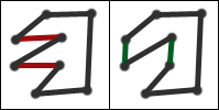 Think of a cycle not as a list of cities to visit but as a cycle in a graph. It may be that we could shorten the length of the cycle by "swapping" two edges. See the example.
You can probably convince yourself that given two edges (not necessarily separated by a single edge like in the above diagram) which do not share vertices, there is only one way to delete them and create two new edges so that the cycle is preserved. Imagine a cycle such that no matter what pair of edges we select we can not improve the length in this manner. Since we can't make the cycle better by swapping any two edges, we'll call such a cycle "two-optimized". Obviously the optimal cycle is two-optimized, but there are plenty of non-optimal cycles which are two-optimized as well.
There are a finite number of edges in a cycle. There are also a finite number of pairs of edges in a cycle. So, what we should do is look through all pairs of edges, and find which pair (if any) can be swapped so as to reduce the total length by the greatest amount. Then we can swap those edges and try again. When we can't swap any more edges (this has to happen eventually), we have made our cycle two-optimized, using a deterministic algorithm. We can uninventively call the process of making a graph two-optimized "two-optimization".
There is one way that two-optimization may be enhanced, but I have not tried it. It is not necessarily so that picking the pair of edges whose swapping reduces the length by the greatest amount is best. Perhaps we should recursively try all possible edge-swaps which lead to an improvement, and select the best two-optimized path which is eventually created. This would lead to a large increase in the computational power needed, but it is still a deterministic algorithm and not horrendously bad. (Since we still retain the constraint that every edge-swap must reduce the total length, things are kept neat. If we recursively tried all edge swaps, we would eventually find the optimal path after an exponential number of calculations!)
Three-optimization.
We can also iterate through all triples of edges and see which edge rearrangement leads to the greatest reduction in cycle length, perform that edge rearrangement, and then repeat until it can't be done any more. This process is obviously three-optimization (and the optimal cycle is once again by definition three-optimized), and it has the potential to improve a cycle which is already two-optimized. Of course, it carries a greater cost in both computational power and in algorithm complexity. I believe that if the three original edges are deleted, that there are only two ways to create three new edges such that the cycle is preserved (i.e. it is not split up into separate loops), but I may be incorrect.
There is also four-optimization and higher levels (all of which I have not tried), which are increasingly costly and offer diminishing returns.
The deterministic algorithm.
Create all NN paths. Two-optimize, then three-optimize all of them. Select the best one.
The Earth falling into the Sun
(Not related to coursework.)
Suppose that an asteroid with the Earth's mass moving at 30 km/sec hits the Earth tangential to its orbit, zeroing out the Earth's tangential velocity. How long would it take the Earth to fall into the Sun? [We make several approximations here: most notably, the mass of the asteroid and Earth combined are not significant compared to the mass of the Sun.]
This might seem to be an easy problem, but as the Earth falls into the Sun it undergoes increasing acceleration. This leads to a differential equation which can be solved, but not without some work.
Recall Kepler's third law, the Law of Periods: The square of the period of any planet about the Sun is proportional to the cube of the planet's mean distance from the Sun. We can prove this result for circular orbits easily. Recall that the centripetal force required to keep an object of mass m moving at velocity v in a circle of radius r is m * v2 / r. Also recall that angular speed ω is v / r, and that the period T is 2 * π / ω. As the gravitational force G * MSun * MEarth / r 2 is equal to the centripetal force, we have:
G * MSun * MEarth / r 2 = MEarth * v2 / r
G * MSun / r 2 = v2 / r
G * MSun / r 2 = ω2 * r
G * MSun / r 3 = ω2
G * MSun / r 3 = (2 * π / T)2
G * MSun / r 3 = 4 * π2 / T2
T2 = 4 * π2 * r 3 / (G * MSun)
We can prove that the same equation holds for elliptical orbits, replacing the radius r by the semimajor axis a:
T2 = 4 * π2 * a 3 / (G * MSun)
Note that this makes us happy - it confirms Kepler's empirical law, and is independent of the eccentricity of the orbit - it holds for both circular ones and extremely long, narrow orbits.
In this problem, we can view the Earth as traveling on an infinitely skinny elliptical orbit, with the Sun at one focus at one end of the orbit and the Earth starting at the other end. The major axis of this orbit is the distance r from the Earth to the Sun, so the semimajor axis is r / 2. In addition, the Earth is only going to execute half of this orbit, so we want to find not T but T / 2.
T = √[4 * π2 * (r / 2)3 / (G * MSun)]
T = √[4 * π2 * r3 / (8 * G * MSun)]
T = 2 * π * √[r3 / (8 * G * MSun)]
T / 2 = π * √[r3 / (8 * G * MSun)]
In SI units, G is 6.67259 * 10−11, MSun is 1.989 * 1030, and the Earth-Sun distance is about 1.496 * 1011. So, we get:
π * √[(1.496 * 1011)3 / (8 * 6.67259 * 10−11 * 1.989 * 1030)] = 5578760
5578760 seconds is 64.57 days.
This problem can also easily be solved computationally:
#include <stdio.h>

/* SI units */
#define RESOLUTION 1
#define SUNRADIUS 695000000
#define SUNMASS 1.989e30
#define BIGG 6.6739e-11
#define EARTHORBITRADIUS 1.496e11

int main(void) {
    double x = EARTHORBITRADIUS;
    double v = 0;
    double t = 0;

    while (x > SUNRADIUS) { /* Not x > 0, beware */
        t += RESOLUTION;
        v -= BIGG * SUNMASS * RESOLUTION / (x * x);
        x += v * RESOLUTION;
    }
    printf("CRASH! Time: %f days, Velocity: %f m/s\n", t / 86400, -v);
    return 0;
}
The computational method indicates that the Earth achieves a significant velocity at the end, a small fraction of the speed of light.
Triple inversion with logic gates
(Not related to coursework.)
This problem is found in found in HAKMEM Item 19.
PROBLEM: Given three inputs A, B, C, and arbitrary numbers of two-input AND gates and two-input OR gates, but only two NOT gates, synthesize separately the NOT-A, NOT-B, and NOT-C signals.
SOLUTION: The notation is X Y for X AND Y; X + Y for X OR Y; /X for NOT X.
So, given the three inputs A, B, C:
- A B.
- A C.
- B C.
- A + B.
- A + C.
- B + C.
- (1) C = A B C.
- (4) + C = A + B + C.
- (4) C = A C + B C.
- (1) + (9) = A B + A C + B C.
- /(10) = /A /B + /B /C + /A /C.
- (7) + (11) = A B C + /A /B + /B /C + /A /C.
- (12) (8) = A B C + A /B /C + /A B /C + /A /B C.
- /(13) = A B /C + A /B C + /A B C + /A /B /C.
- (1) + (11) = A B + /A /B + /B /C + /A /C.
- (4) (11) = A /B /C + /A B /C.
- (2) + (11) = /A /B + /B /C + /A /C + A C.
- (5) (11) = A /B /C + /A /B C.
- (3) + (11) = /A /B + /B /C + /A /C + B C.
- (6) (11) = /A B /C + /A /B C.
- (14) + (16) = A /B + /A B + /C.
- (14) + (18) = A /C + /A C + /B.
- (14) + (20) = B /C + /B C + /A.
- (15) (21) = /C.
- (17) (22) = /B.
- (19) (23) = /A.
Iteration with lambda functions.
(Not related to coursework.)
In Scheme, functions are first-class datatypes and lambda functions are unnamed functions. At first glance, it appears impossible for a lambda function to call itself, because it has no name. Yet, we can perform iterative computations with lambda functions if we wish, entirely avoiding the use of define.
First, how might we write an iterative factorial function? (For the time being, I will ignore good style and not provide wrapper functions. A factorial function really should have the interface (factorial 10) and should not require extra arguments set to certain values by the user.)
(define (iterative-factorial n result)
  (if (= n 1)
      result
      (iterative-factorial (- n 1) (* result n))
  )
)

(iterative-factorial 10 1) ;; Computes 10!
iterative-factorial takes two arguments, n and result. The user passes a positive integer of his liking as n and 1 as the initial result. iterative-factorial then tests if the computation is done (when n is equal to 1), in which case it returns result. Otherwise, it calls itself, appropriately updating n and appropriately updating the result.
Now, let's create a proto-factorial function.
(define (proto-factorial check-if-done update-n update-result n result)
        (cond (check-if-done (= n 1)     )
              (update-n      (- n 1)     )
              (update-result (* result n))
        )
)
proto-factorial takes three behavior switches. The switch for the desired behavior should be set to #t with the others set to #f. We can call it like:
> (proto-factorial #f #f #t 10 1) ;; If n is 10 and result is 1, what will be the next result?
10
> (proto-factorial #f #t #f 10 1) ;; If n is 10, what will be the next n?
9
> (proto-factorial #t #f #f 10 1) ;; If n is 10, is it time to stop the iteration?
#f
Of course, we are simply using syntatic sugar in proto-factorial's definition. It is equivalent to:
(define proto-factorial
  (lambda (check-if-done update-n update-result n result)
          (cond (check-if-done (= n 1)     )
                (update-n      (- n 1)     )
                (update-result (* result n))
          )
  )
)
Now, we need some sort of master function which will repeatedly call proto-factorial.
(define (recurse fxn done n result)
    (if done
        result
        (recurse
          fxn                     ;; Hand the function down
          (fxn #t #f #f n result) ;; Ask whether we are done
          (fxn #f #t #f n result) ;; Ask what the new n should be
          (fxn #f #f #t n result) ;; Ask what the new result should be
        )
    )
)
So, calling (recurse proto-factorial #f 10 1) gives us 10! like we expect. However, recurse calls itself by name, which we must eliminate.
(define (proto-recurse fxn done n result prfxn)
    (if done
        result
        (prfxn
          fxn                     ;; Hand the function down
          (fxn #t #f #f n result) ;; Ask whether we are done
          (fxn #f #t #f n result) ;; Ask what the new n should be
          (fxn #f #f #t n result) ;; Ask what the new result should be
          prfxn                   ;; Hand prfxn down
        )
    )
)
proto-recurse is just like recurse, but it takes an additional argument, prfxn. Instead of calling itself with the updated n, updated result, etc, it calls prfxn on those things. The intent is that prfxn will be proto-recurse itself.
Now we can call (proto-recurse proto-factorial #f 10 1 proto-recurse) and compute 10! which is excellent. We could write proto-recurse as a lambda function, and it would still work. This is because proto-recurse never calls itself, it only executes prfxn. However, things are still not pretty: we would have to write out the lambda function form of proto-recurse twice, once to execute it and once to pass it to itself. Instead, we could use a let to appropriately duplicate the definition. And we can write let in terms of lambda, yay!
(
  (lambda (thing-to-duplicate)
    ;; Just like:
    ;; (proto-recurse proto-factorial #f 10 1 proto-recurse)
    (thing-to-duplicate proto-factorial #f 10 1 thing-to-duplicate)
  )
  ;; proto-recurse:
  (lambda (fxn done n result prfxn)
     (if done
         result
          (prfxn
            fxn                     ;; Hand the function down
            (fxn #t #f #f n result) ;; Ask whether we are done
            (fxn #f #t #f n result) ;; Ask what the new n should be
            (fxn #f #f #t n result) ;; Ask what the new result should be
            prfxn                   ;; Hand prfxn down
          )
      )
  )
)
Now we can just substitute in proto-factorial's definition, since it's a lambda function too.
(
  (lambda (thing-to-duplicate)
    (thing-to-duplicate
      ;; proto-factorial:
      (lambda (check-if-done update-n update-result n result)
        (cond (check-if-done (= n 1)     )
              (update-n      (- n 1)     )
              (update-result (* result n))
        )
      )
      #f
      10
      1
      thing-to-duplicate
    )
  )
  ;; proto-recurse:
  (lambda (fxn done n result prfxn)
     (if done
         result
          (prfxn
            fxn                     ;; Hand the function down
            (fxn #t #f #f n result) ;; Ask whether we are done
            (fxn #f #t #f n result) ;; Ask what the new n should be
            (fxn #f #f #t n result) ;; Ask what the new result should be
            prfxn                   ;; Hand prfxn down
          )
      )
  )
)
And finally we can wrap up the whole thing in a nice bow:
(define factorial
  (lambda (number)
    (
      (lambda (thing-to-duplicate)
        (thing-to-duplicate
          ;; proto-factorial:
          (lambda (check-if-done update-n update-result n result)
            (cond (check-if-done (= n 1)     )
                  (update-n      (- n 1)     )
                  (update-result (* result n))
            )
          )
          #f
          number
          1
          thing-to-duplicate
        )
      )
      ;; proto-recurse:
      (lambda (fxn done n result prfxn)
         (if done
             result
              (prfxn
                fxn                     ;; Hand the function down
                (fxn #t #f #f n result) ;; Ask whether we are done
                (fxn #f #t #f n result) ;; Ask what the new n should be
                (fxn #f #f #t n result) ;; Ask what the new result should be
                prfxn                   ;; Hand prfxn down
              )
          )
      )
    )
  )
)
Now we can compute (factorial 10) whenever we please. (Or, we could write out that huge lambda function in place of factorial, if define scares us.)
Of course, all that complicated machinery really isn't necessary. With these principles in mind, we can develop a general way to allow lambda functions to recurse on themselves. This computes factorials:
(
  (lambda (f . data)
    (apply f (cons f data))
  )
  (lambda (fxn n)
    (if (= 0 n)
        1
        (* n (fxn fxn (- n 1)))
    )
  )
  10
)
And this is a recursive multiply function:
(
  (lambda (f . data)
    (apply f (cons f data))
  )
  (lambda (fxn a b)
    (if (= 0 b)
        0
        (+ a (fxn fxn a (- b 1)))
    )
  )
  10
  15
)
This takes advantage of Scheme varargs, cons, and apply.
https://nuwen.net/work.html (updated a long time ago)
Stephan T. Lavavej
Home: stl@nuwen.net
Work: stl@microsoft.com
This is my personal website. I work for Microsoft, but I don't speak for them.