bwtzip - nuwen.net
Not all bits have equal value
bwtzip: A Linear-Time Portable Research-Grade Universal Data Compressor
bwtzip is an ongoing project, distributed under the GNU General Public License, to implement a Burrows-Wheeler compressor in standard, portable C++. It is research-grade in that it is highly modularized and abstracted, so that it is simple to swap out parts of the compressor without affecting anything else. This makes it easy to experiment with different algorithms at different stages of compression. It's also research-grade in the sense that little attention has been given to microoptimization; production-grade code would look very different. bwtzip is universal in that it can be used with arbitrary binary files and is always lossless. Furthermore, bwtzip and bwtunzip both are true linear-time algorithms.
Status - 21st Century Compression, 22nd Century Memory Usage
- All of the necessary algorithms for Burrows-Wheeler compression have been implemented in bwtzip.
- There are no known bugs in bwtzip.
- bwtzip generally produces smaller compressed output than bzip2 and ZIP.
- There are still several issues to be resolved before bwtzip can be used widely, explained in the Issues section. Chief among them is bwtzip's memory usage.
Download
bwtzip.zip (238 KB) : C++ source code and Win32 executables for bwtzip.
To compress a given file, say jargon.html, execute bwtzip jargon.html jargon.bwt and the output file jargon.bwt will be produced. To decompress a given file, execute bwtunzip jargon.bwt jargon.out which will produce the output file jargon.out. bwtzip is not meant for general use yet. Do not trust bwtzip to correctly archive any of your data and do not expect that future versions of bwtzip will understand files that previous versions created.
Efficiency
A direct comparison in terms of performance of bwtzip to publicly available compressors such as zlib or bzip2 is not particularly enlightening as bwtzip is only research-grade code. However, the efficiency of bwtzip can be analyzed and compared to other compressors.
I have created three large corpuses to compare compressors with: the Large English Text Corpus, the Large Source Code Corpus, and the Human Genome Corpus. (Their contents are listed here.)
| Large English Text Corpus |
| Compression Method |
Size (Bytes) | Output Bits
Per Input Byte |
| Original: |
84,683,776 | 8.000 |
| XP Integrated ZIP: |
31,581,308 | 2.983 |
| gzip 1.2.4 --best: |
30,716,422 | 2.902 |
| WinACE 2.2 [Max, 4 MB]: |
24,154,354 | 2.282 |
| bzip2 1.0.2 (900 KB): |
22,320,624 | 2.109 |
| bwtzip (900 KB): |
22,021,513 | 2.080 |
| bwtzip (5 MB): |
20,354,229 | 1.923 |
| bwtzip (15 MB): |
19,839,276 | 1.874 |
| RAR 3.11 -m5: |
18,951,292 | 1.790 |
|
| Large Source Code Corpus |
| Method |
Size | Bits/Byte |
| Original: |
286,834,688 | 8.000 |
| ZIP: |
62,776,873 | 1.751 |
| gzip: |
61,063,845 | 1.703 |
| bwtzip (900 KB): |
49,232,746 | 1.373 |
| bzip2: |
47,999,290 | 1.339 |
| bwtzip (5 MB): |
44,919,628 | 1.253 |
| WinACE: |
44,745,014 | 1.248 |
| bwtzip (15 MB): |
43,414,032 | 1.211 |
| bwtzip (25 MB): |
43,153,662 | 1.204 |
| RAR: |
39,586,669 | 1.104 |
|
| Human Genome Corpus |
| Method |
Size | Bits/Byte |
| Original: |
3,358,188,544 | 8.000 |
| ZIP: |
867,363,935* | 2.066 |
| gzip: |
799,270,472 | 1.904 |
| bzip2: |
759,562,051 | 1.809 |
| WinACE: |
755,978,596 | 1.801 |
| bwtzip (900 KB): |
729,626,896 | 1.738 |
| bwtzip (5 MB): |
717,566,495 | 1.709 |
| bwtzip (15 MB): |
709,462,877 | 1.690 |
| RAR: |
679,128,824 | 1.618 |
|
(Values in parentheses refer to chunk size.)
* XP Integrated ZIP could not compress the entire TAR file or all of the files simultaneously. Hence, the files were compressed individually and their sizes were added together.
How should these tables be interpreted? ZIP and gzip are both 1970s-era dictionary compressors, and thus perform similarly. bzip2 and bwtzip are 1990s-era Burrows-Wheeler compressors, but bwtzip uses more advanced algorithms. ACE uses a proprietary (read: bletcherous) algorithm. RAR also uses a proprietary (read: bletcherous) algorithm; it is self-admittedly PPM-based.
A common question arises: why not use Prediction by Partial Matching? PPM is the highest-efficiency compression algorithm yet developed, and it is conjectured that the best PPM implementations will always be more efficient than the best BWT implementations. This does not mean that PPM is universally superior to BWT. BWT is attractive because it is low complexity as well as (fairly) easily implemented.
RAR specifically should not be used because its algorithm is proprietary. The same goes for ACE. We're better than that. No matter how well they compress, they're not worth using. If you don't get this point, and are stuck thinking, "but they're more efficient!", you can pack up your bags and go home. Proprietary algorithms are disgusting. We don't need them.
I provide results for RAR and ACE here merely to be complete. The real algorithms to be considered are the ones with open source: gzip, bzip2, bwtzip. (XP Integrated ZIP is not open source, but zlib is, and they perform similarly.) So, which compressor is the "best"? Obviously, not the 1970s-era dictionary compressors. It is no longer worthwhile to endure their inefficiency even though they have extremely high speed and extremely low memory usage. We're left with bzip2 and bwtzip, the Burrows-Wheeler compressors. And note that bwtzip allows the entire human genome to be put on a single CD, unlike all the other open source algorithms here.
bwtzip defeats bzip2 and the dictionary compressors even when small chunk sizes are used, with one exception: bzip2 with 900 KB chunks performs better on the Large Source Code Corpus than bwtzip with 900 KB chunks. The reason for this is unclear; I believe it has something to do with bzip2's presort RLE.
With bwtzip's current implementation of the Ukkonen suffix tree algorithm, I believe that 5 MB is the most natural chunk size to use. I think you'll agree that bwtzip is a significant improvement over bzip2 and ZIP.
Frequently Asked Questions
- Q: Is bwtzip compatible with [insert another compressor here; e.g. ZIP]?
- A: No. bwtzip does not produce output that anything else can understand; bwtzip cannot understand output produced by anything else. This is because bwtzip uses new, advanced algorithms not found in ZIP, gzip, or bzip2.
- Q: What is chunk size?
- A: A setting that changes bwtzip's compression efficiency. It is an inherent feature of any Burrows-Wheeler compressor. The algorithm is designed to work on a single block of data. If your file is 10 gigabytes, it may be a bad idea to work on all of it in memory at once. Thus, a Burrows-Wheeler compressor must break up a long file into separate parts (chunks). These chunks are then processed independently. The decompressor then integrates everything together. Controlling how large the chunks are has a few effects.
Larger chunks lead to...
- Higher compression. If the algorithm can see more data at once, it can find more redundancy.
- More memory used during compression. All algorithms ordinarily used to perform the BWT use some constant multiple of the chunk size for temporary memory.
- Slower compression for nonlinear algorithms. This is not true of linear algorithms, such as bwtzip's Ukkonen suffix trees.
- More memory used during decompression. The decompressor also uses some constant multiple of the chunk size for temporary memory. However, this multiple is significantly less than that for the compressor, so ordinarily decompression memory usage is not a consideration. Chunk size has little effect on decompression time, as the algorithm is always linear.
- Q: How can you ever decompress something? Will there ever be a bwtunzip?
- A: bwtunzip is part of the bwtzip project. The two are developed synchronously, since the compressor has to produce output that the decompressor can understand. bwtunzip doesn't get as much attention as bwtzip because its algorithms are simply the mirror image of the compressor. However, any improvements to bwtunzip's performance would be welcome.
- Q: I'm not a programmer. All these files confuse me. What do I need and what can I delete?
- A: You only need the EXE files. The CC, HH, and TXT files are unnecessary if you don't care about the source code.
- Q: How can I uninstall bwtzip?
- A: Simply delete bwtzip's EXE files. bwtzip makes no changes to your system. It's the way programs should behave.
- Q: Is bwtzip available for other platforms?
- A: Sure. My only interest is in Win32 and Linux, but the source code is reasonably portable and should work on all sorts of other platforms. If you use Linux, compile bwtzip yourself. If you've found a portability problem in bwtzip, I'd like to hear about it. However, I have no sympathy for systems that have non-8-bit unsigned chars, 16-bit ints, non-32-bit unsigned longs, or non-64-bit unsigned long longs.
- Q: Who has worked on bwtzip?
- A: Stephan T. Lavavej and Joergen Ibsen, in chronological order. I [Stephan] am the original author; I created the bwtzip framework, as well as implementing (and reimplementing) many algorithms. Joergen contributed an adaptive Huffman encoder; his website is www.ibsensoftware.com.
- Q: Can I see the source code?
- A: Of course. bwtzip is distributed under the GNU GPL.
- Q: Can I use the source code in one of my own projects?
- Q: How can I help?
- A: Spread the word, report bugs, or contribute code, in order of increasing difficulty. If you contribute code, it must be GPLed or public domain. It helps immensely if you can follow bwtzip's coding conventions. As for spreading the word, that may be the most helpful thing of all. It's time to create a high-performance, high-efficiency compressor for the twenty-first century, and I think that bwtzip is that compressor. bwtzip is already very efficient; as more people learn about and experiment with bwtzip, we'll make its performance acceptable.
- Q: How do you pronounce bwtzip?
- A: I pronounce it "bee double-you tee zip". It may not be the most euphonic pronunciation, but it works for me. Alternative suggestions I have heard include "beaut zip" (as in beautiful), "boot zip", and "bw00tzip". :-)
- Q: Why the name bwtzip?
- A: I am ridiculously uninventive. bwtzip uses the Burrows-Wheeler Transformation, and it's traditional to give compressors names that end with zip. (pkzip, gzip, bzip2, etc.) Furthermore, no one has ever used the name bwtzip before.
- Q: Can I see the file format?
- A: Yes, but it's not clearly documented. I'm an ardent believer in open file format specifications. It does no good if free reading/writing implementations exist for a file format if the specification is not available to all. (I'm looking at you, Ogg Vorbis.) The golden standard for file format specifications is the Portable Network Graphics standard, which is freely available and readily comprehensible. Unfortunately, bwtzip is not quite there yet. Too much work is going into the algorithms themselves for the file format to be stable. (It changes every time a major revision occurs in the code; different versions of bwtzip usually cannot understand each other.) That said, if you wanted to, you could look at the bwtzip algorithms and figure out the format I use for compressed output. Now, the eventual goal is for bwtzip to go from research-grade to production-grade code without compromising its clarity. Once it settles down, an actual file format can be written down clearly for all to see. It wouldn't take more than a couple of pages; the hardest thing is to describe how the arithmetic compressor works.
The rest of this page explains the algorithms used in bwtzip.
Definitions
We will define an alphabet to be a finite set whose elements are called symbols, and we will define a string (without the C connotations) to be a finite sequence of symbols. [In data compression, the alphabet is the 256 types of bytes (from 0 to 255 inclusive) and the strings are binary files or arrays.] We write down a string A as a0 a1 ... an - 1 where ai is the ith symbol in the string (counting from 0). Additionally, we will define the suffix beginning at i of a string to be Ai = ai ai + 1 ... an - 1 and obviously the suffix beginning at 0 of a string is the string itself. We will define the prefix ending at i of a string to be a0 ... ai and the prefix ending at n - 1 is the string itself. We can define a method of comparing symbols in the alphabet: with bytes, we simply compare their numerical values; with letters, we define A < B < ... < Z. We can then compare two strings A and B 'lexicographically'. If a0 < b0 then A < B. If a0 > b0 then A > B. If a0 = b0 then we compare a1 and b1, if they are the same then we compare a2 and b2, and so forth. (Lexicographic ordering on strings of bytes is the same as dictionary ordering on words.)
The Burrows-Wheeler Transformation
In 1994, the Burrows-Wheeler Transformation (BWT) was developed. This is a radically new compression algorithm which works in a three-step process. First, it losslessly reorders data using the BWT itself, which slightly expands the size of the data. Then, it sends the data through a byte-for-byte Move-to-Front transformation. Finally, it applies an entropy coder, such as Huffman or arithmetic compression. This apparently simplistic process achieves better compression performance than all traditional compressors such as the 1970s-era Lempel-Ziv compressors, and approaches the performance of the best statistical compressors. The BWT relies on lexicographically sorting the circular shifts or the suffixes of a string.
The operation of the BWT can best be explained with an example. We will BWT and reverse-BWT the string STEPHANTLAVAVEJ (note the repetitive substring AVAV). Notes relevant to implementation but not the theoretical operation of the algorithm are in italics.
BWT Example
Input:
STEPHANTLAVAVEJ
Now, we create all circular shifts of this string and list them in order. (In practice, this is done with an array of indexes to positions in the original string.)
Shift:
STEPHANTLAVAVEJ
TEPHANTLAVAVEJS
EPHANTLAVAVEJST
PHANTLAVAVEJSTE
HANTLAVAVEJSTEP
ANTLAVAVEJSTEPH
NTLAVAVEJSTEPHA
TLAVAVEJSTEPHAN
LAVAVEJSTEPHANT
AVAVEJSTEPHANTL
VAVEJSTEPHANTLA
AVEJSTEPHANTLAV
VEJSTEPHANTLAVA
EJSTEPHANTLAVAV
JSTEPHANTLAVAVE
Now, we sort these strings lexicographically. (This is where a bubblesort, quicksort, suffix array sort, suffix tree sort, etc. is used.)
Sort:
ANTLAVAVEJSTEPH
AVAVEJSTEPHANTL
AVEJSTEPHANTLAV
EJSTEPHANTLAVAV
EPHANTLAVAVEJST
HANTLAVAVEJSTEP
JSTEPHANTLAVAVE
LAVAVEJSTEPHANT
NTLAVAVEJSTEPHA
PHANTLAVAVEJSTE
STEPHANTLAVAVEJ
TEPHANTLAVAVEJS
TLAVAVEJSTEPHAN
VAVEJSTEPHANTLA
VEJSTEPHANTLAVA
The output of the BWT is then the last letter of each string in succession, as well as an index to which of those letters is the original first letter of the string. This is a unique choice even if there are multiple copies of that letter in the string (here, there are not - there is only one S in STEPHANTLAVAVEJ). This is called the primary index.
Identify:
ANTLAVAVEJSTEPH Location: 0
AVAVEJSTEPHANTL Location: 1
AVEJSTEPHANTLAV Location: 2
EJSTEPHANTLAVAV Location: 3
EPHANTLAVAVEJST Location: 4
HANTLAVAVEJSTEP Location: 5
JSTEPHANTLAVAVE Location: 6
LAVAVEJSTEPHANT Location: 7
NTLAVAVEJSTEPHA Location: 8
PHANTLAVAVEJSTE Location: 9
STEPHANTLAVAVEJ Location: 10
TEPHANTLAVAVEJS Location: 11 <== The original first letter
TLAVAVEJSTEPHAN Location: 12
VAVEJSTEPHANTLA Location: 13
VEJSTEPHANTLAVA Location: 14
Output:
HLVVTPETAEJSNAA, 11
Reverse-BWT Example
Note that the output of the BWT is the last column in the sorted matrix of letters produced. Call that column L. If we sort the output of the BWT, we will get the first column of the sorted matrix, which we will call column F. (This sort can be done in O(N) time, as symbols are indistinguishable: simply make one pass over the output of the BWT to count the frequencies with which each symbol occurs, and then in another pass write the appropriate numbers of symbols in order.)
Sort:
AAAEEHJLNPSTTVV
Now, we will write the L and F strings side by side, along with indexes:
Index: 0 1 2 3 4 5 6 7 8 9 10 11 12 13 14
L:     H L V V T P E T A E J  S  N  A  A
F:     A A A E E H J L N P S  T  T  V  V
Now, we must produce a "transformation vector". If the original string was of length N, then the transformation vector is a list of N indexes. To compute the ith entry in the transformation vector, T[i], we look at the ith letter of the F string. We then find how many times the letter occurs up to and including that position in the F string - that is to say, if F[i] is a Z, we must determine whether that is the first Z in F, or the second, etc. Suppose we find that it is the jth occurrence of that letter. We then scan through the L string to find the jth occurrence of that letter. When we find it, the position of this letter in L is recorded as the value of T[i].
Recover T:
F[0]  is the 1st A in F. L[8]  is the 1st A in L. T[0]  = 8
F[1]  is the 2nd A in F. L[13] is the 2nd A in L. T[1]  = 13
F[2]  is the 3rd A in F. L[14] is the 3rd A in L. T[2]  = 14
F[3]  is the 1st E in F. L[6]  is the 1st E in L. T[3]  = 6
F[4]  is the 2nd E in F. L[9]  is the 2nd E in L. T[4]  = 9
F[5]  is the 1st H in F. L[0]  is the 1st H in L. T[5]  = 0
F[6]  is the 1st J in F. L[10] is the 1st J in L. T[6]  = 10
F[7]  is the 1st L in F. L[1]  is the 1st L in L. T[7]  = 1
F[8]  is the 1st N in F. L[12] is the 1st N in L. T[8]  = 12
F[9]  is the 1st P in F. L[5]  is the 1st P in L. T[9]  = 5
F[10] is the 1st S in F. L[11] is the 1st S in L. T[10] = 11
F[11] is the 1st T in F. L[4]  is the 1st T in L. T[11] = 4
F[12] is the 2nd T in F. L[7]  is the 2nd T in L. T[12] = 7
F[13] is the 1st V in F. L[2]  is the 1st V in L. T[13] = 2
F[14] is the 2nd V in F. L[3]  is the 2nd V in L. T[14] = 3
Now, to restore the original string, we need to use the primary index. We initialize an index to the value of the primary index. Then we look up L[index], and set the index to T[index], and repeat until we reach the primary index again.
Decode:
Index: 0 1  2  3 4 5 6  7 8  9 10 11 12 13 14
L:     H L  V  V T P E  T A  E J  S  N  A  A
T:     8 13 14 6 9 0 10 1 12 5 11 4  7  2  3

Read primary index. Value: 11
Index = 11  L[11] = S   T[11] = 4
Index = 4   L[4]  = T   T[4]  = 9
Index = 9   L[9]  = E   T[9]  = 5
Index = 5   L[5]  = P   T[5]  = 0
Index = 0   L[0]  = H   T[0]  = 8
Index = 8   L[8]  = A   T[8]  = 12
Index = 12  L[12] = N   T[12] = 7
Index = 7   L[7]  = T   T[7]  = 1
Index = 1   L[1]  = L   T[1]  = 13
Index = 13  L[13] = A   T[13] = 2
Index = 2   L[2]  = V   T[2]  = 14
Index = 14  L[14] = A   T[14] = 3
Index = 3   L[3]  = V   T[3]  = 6
Index = 6   L[6]  = E   T[6]  = 10
Index = 10  L[10] = J   T[10] = 11
Index = 11  Primary index reached, end of string.
Output:
STEPHANTLAVAVEJ
Long BWT Example
Here is an example of what happens when the BWT is applied to a longer text. What it does is much clearer to see when there's more data.
The original text is the introduction to The Lord of the Rings by J.R.R. Tolkien. To make things more visible in the transformed text, I have replaced the spaces in the original passage with underscores and I have replaced newlines with # symbols. To the end of the text I have appended a sentinel, the $ symbol. I present the text wrapped at 80 characters, but it was treated as one long string of symbols while being transformed.
Three_Rings_for_the_Elven-kings_under_the_sky,#Seven_for_the_Dwarf-lords_in_the
ir_halls_of_stone,#Nine_for_Mortal_Men_doomed_to_die,#One_for_the_Dark_Lord_on_
his_dark_throne#In_the_Land_of_Mordor_where_the_Shadows_lie.#One_Ring_to_rule_t
hem_all,_One_Ring_to_find_them,#One_Ring_to_bring_them_all_and_in_the_darkness_
bind_them#In_the_Land_of_Mordor_where_the_Shadows_lie.#$
And here is the transformed text. Again, it is wrapped at 80 characters for display purposes only. I have not recorded the position of the original first symbol.
.me,,.,,#emeylnfee___##_______##_##____#__$eeeeeklffr,eeeeeemmlsoseonoeensrndss
sddsdoefrrrnneenrnddegkgdggsrrhht__h_LLwDdd__nnnrnne__n__rraarnniiihhhhhnnnehhh
nnhrrlmrhhhhhvMvdhhnSrooo_____nnnnnnSS_ttttttttttttttww_Ttdll__bfNrRRRRkehrr-rs
lalu__aaa-lEeeeeoeeeoIIiiaaaiiuooOOOiOkiiiiiitttt___o_rtdffffddLMMlMddoioooeooo
oooeehabaaaho_sigdwwlg_e_r___________________sr_leD__ook
Note the long runs of symbols which are produced. Near the beginning of the transformed text, _ and # are clustered together. Near the end of the transformed text, there is a large run of underscores. The M's, O's, and R's are brought together; I preserved the uppercase/lowercase distinctions in the original text so that this effect would be apparent.
Asymptotic Time Complexity
The asymptotic time complexities of the Burrows-Wheeler Transformation and its reverse are not immediately apparent. The real difficulty in the forward transformation is the sorting stage. Once that is accomplished, producing the output of the transformation as well as the primary index is obviously linear time.
We are all taught in introductory computer science courses that sorting, in general, requires O(N log N) comparisons. Since we are not sorting integers here, but suffixes of an N-symbol string, comparing two suffixes lexicographically takes O(N) time. Thus, naively sorting suffixes takes O(N2 log N) time! In fact, things are not quite that bad. The Manber-Myers algorithm takes O(N log N) time to sort the suffixes of a string.
Things can be done even faster, though. It is a surprising fact that the BWT sort can be done in linear time! The objects being sorted in the BWT are not unrelated - they are all derived from the same original string. It is possible to read in the original string and maintain a complex data structure in memory, carefully building it up as the string is read in, and finally traversing the data structure in linear time to accomplish the Burrows-Wheeler sort. This linear-time algorithm, known by the name of its data structure, the suffix tree, was well-known before the development of the Burrows-Wheeler algorithm in 1994. (See an Introduction to Suffix Trees below.)
Suffix tree algorithms are fundamentally space-greedy. Even the most optimized suffix tree algorithms consume approximately 20N bytes of temporary storage to transform N bytes in the worst case. This space consumption can be problematic in limited memory systems, so nonlinear algorithms have been used for the BWT:
- The Manber-Myers suffix array algorithm (also implemented in bwtzip), runs in O(N log N) worst case time and requires 8N bytes of space, but is considerably slower than suffix trees (on the order of 3x to 10x slower).
- The Bentley-Sedgewick algorithm is based on quicksort, requires only 5N bytes of space, and is rather fast in the average case. However, it is extremely slow in the worst case, which occurs when the input sequence contains long repeated substrings. bzip2 implements the Bentley-Sedgewick algorithm.
- The Larsson-Sadakane algorithm runs in O(N log N) worst case time and uses 8N bytes of space. It is reported to be only slightly slower than a suffix tree algorithm.
Of course, any plain old sort which correctly orders the strings can be used to compute the BWT (a bubblesort was used in the earliest versions of bwtzip), but a plain old sort will not exploit the redundant nature of the strings being sorted nearly as well as more specialized algorithms do.
It is not clear on first glance what the asymptotic time complexity of the reverse-BWT is. Upon closer examination, even the naive algorithm presented above (which can be performed by hand) can be implemented in a linear-time fashion. There are even clearer versions of the algorithm which are very obviously linear time. (One of these is implemented in bwtzip.)
All of the other algorithms in a Burrows-Wheeler compressor (MTF, ZLE, Huffman, Arithmetic) and all of their reverses are linear time.
Circular Shifts = Suffixes
In the Burrows-Wheeler Transform, circular shifts of the input string are sorted. Yet, I mentioned that this can also be accomplished by sorting suffixes. Indeed, we can view suffixes and circular shifts as being nearly interchangeable: uniquely associate any suffix ai ... an - 1 with the circular shift ai ... an - 1 a0 ... ai - 1. However, while we can associate suffixes and circular shifts in this fashion, it is not literally true that sorting the suffixes of a string X is identical to sorting the circular shifts of X. This is because one suffix S1 of X may be the prefix of another suffix S2 of X. When comparing S1 to S2, all of the symbols in S1 will compare identical to the first symbols of S2 (this is what it means to be a prefix, after all), and then we will be out of symbols in S1. Since S1 is shorter than S2, we will declare S1 < S2. If we were viewing S1 and S2 as circular shifts, then we would not run out of symbols - we would wrap around, and begin comparing the beginning of X to the remaining symbols in S2. It could very well be that the next symbols in S2 are less than the symbols at the beginning of X, and thus the true ordering would be S2 < S1. In effect, suffixes do not have enough information to be properly ordered by the Burrows-Wheeler lexicographic sort.
This problem is caused whenever one suffix is the prefix of another suffix. In that case, the comparison "runs off the end". Running off the end is never a problem with circular shifts (since there is no end), but it is a problem with suffixes. Note that if no suffix is the prefix of any other suffix, then we never have a problem - all comparisons will end before we run off the end of any suffix, and it will be just as if we were sorting circular shifts.
You may say, how often does it happen that one suffix of a string is the prefix of another suffix of that string? After all, that sounds rather funny, so it can't happen that often. Maybe we can just special-case it and forget all about it. Alas, this is not so. Suppose our intrepid string X ends in a symbol c. If c occurs anywhere else in X, observe what happens. One suffix of X is just its last symbol, c. Another suffix of X starts at the second occurrence of this symbol, and is c.... Ah, and now one suffix is the prefix of another suffix. So, this happens a lot.
Yet, this gives us the hint we need to eliminate this situation for good. Suppose we take an arbitrary string X. Let us add a special new symbol to the end of X. We will call this symbol the sentinel, and it will be different from all the other symbols that occur in X. We can do this even if X uses all the symbols in the alphabet - we'll simply expand the alphabet to include a new symbol, and make that the sentinel. Traditionally, the sentinel is represented by $. When working with bytes, the sentinel is often fictional byte 256 (remember that the normal bytes range from 0 to 255 inclusive). So, if X = a0 ... an - 1, then let's call our augmented string Y, and Y = a0 ... an - 1 $ with $ != ai for any i.
Proof by contradiction: Suppose that we have two suffixes S1 and S2 of Y and that S1 is a proper prefix of S2. (Proper means that they are nonidentical.) Call the length of S1 to be Q and the length of S2 to be R. We know that Q < R, so the symbol at Q - 1 in S2 is not the last symbol in S2. The symbol at position Q - 1 in S1 is the sentinel, $. Since S1 is a proper prefix of S2, this means that the symbol at position Q - 1 in S2 is the sentinel. Contradiction! We have seen the sentinel occurring in S2, and it is not the last symbol in S2. Yet by definition the sentinel occurs at and only at the end of any suffix of Y. Hence, our assumption that S1 is a proper prefix of S2 is at fault.
This gives us the power to fix our problem. Sorting suffixes is identical to sorting circular shifts as long as the string has a sentinel character tacked onto it. When two suffixes are being compared, you will hit the sentinel in one suffix before you run off the end of that suffix, and since the sentinel will be different then the corresponding character in the other suffix, your comparison will resolve right then and there without falling off the end. (You have to define how the sentinel character compares to the other, normal characters - usually, the sentinel is said to be lexicographically greater than everything else, but as long as you are consistent, the precise definition is irrelevant.) It's easy to always add a sentinel character, even if the string by chance ends in a unique character. It doesn't hurt anything. Thus, we can tack on a sentinel, sort suffixes, and produce the Burrows-Wheeler transformed version of the augmented string. (Of course, if you can't actually write down the sentinel in your machine's alphabet, you will need to play funny games to simulate being able to store 257 types of bytes.) Then you can un-transform the result, and strip off the sentinel. Compression is harmed very insignificantly (perhaps a half-dozen bytes), and the increased ease of sorting is well worth it.
The Move-to-Front Transformation
The Move-to-Front transformation is conceptually simple. It is a byte-for-byte streaming transformation, meaning that it neither expands nor compresses the data given to it, and every byte put into the algorithm produces a byte of output. This byte of output can then be decoded without referring to any bytes further ahead in the data.
This is all that is necessary to implement the algorithm: Input a byte B into the MTF algorithm. The output of the MTF algorithm is the number of distinct other bytes that have appeared since the last occurrence of B. Before the algorithm receives any bytes, it is implicitly assumed (by both the forward and the reverse transformation) that byte 0 has occurred most recently, that byte 1 has occurred second most recently, and so forth.
In practice, this is done not by scanning behind in the datastream and counting the number of distinct other bytes that have appeared. Instead, the program remembers which is the most recently seen symbol, the second most recently seen symbol, etc. Thus, we can talk about a symbol being in "position 0" (that would be the most recently seen symbol), "position 1" (the second most recently seen symbol), etc. So, in practice, we maintain an array containing the 256 types of bytes. We can change the order of the bytes in the array to reflect which bytes have been seen more recently. We initialize this array such that the nth most recently seen byte is n. (Note that we're counting starting from zero.) The reverse-MTF algorithm also maintains such an array, which is initialized identically.
The MTF algorithm then operates byte-by-byte upon the input. We first read a byte. Then we determine its location in the array and write that location to the output. (If we choose to do the transformation "in place", we just overwrite the input byte.) We then must update the array to take into account the fact that a new byte has appeared. If the byte was not already in position 0 (most recently seen), we need to remove the byte from its current location, move all the bytes which used to be ahead of it in the array to one higher position each, and then put that byte in position 0.
If you're unfamiliar with size_t, it's just a data type which can hold locations in an array.
If you're unfamiliar with my Bcells, they act just like arrays of unsigned char, except that they have more abilities. If you have a Bcell named cell, you can ask it where the byte uc first appears. We can get this location with cell.find(uc) (in C, we would write it find(cell, uc) - I apologize if object-oriented programming is unfamiliar to you). We can additionally move chunks of bytes around in a Bcell. If we want to move n bytes starting from s to locations starting at d, we can use cell.move(n, s, d).
So, with that in mind, here's the code to do MTF.
Bcell list("MTF Array", 256);    // Bcells have names; this one is named "MTF Array" and can hold 256 bytes

for (int n = 0; n < 256; n++) { // Initialize the list
    list[n] = n;
}

for (size_t n = 0; n < cell.size; n++) {    // For every element in the Bcell cell
    unsigned char uc, out;

    uc = cell[st];            // Input byte
    out = list.find(uc);      // Where is it in the array?
    cell[st] = out;           // Write that back
    if (out != 0) {           // If the byte read isn't in position 0
        list.move(out, 0, 1); // Take the bytes at positions 0, ... , out - 1 and move them to 1, ..., out
        list[0] = uc;         // Put the byte in position 0
    }
}
The reverse algorithm initializes list identically. When it reads an MTF-transformed byte, it determines what resides at that location in list. (That is to say, if it reads a 3, it looks up what character is in position 3.) It then outputs that, and appropriately updates list.
Bcell list("MTF Array", 256);    // Bcells have names; this one is named "MTF Array" and can hold 256 bytes

for (int n = 0; n < 256; n++) { // Initialize the list
    list[n] = n;
}

for (size_t n = 0; n < cell.size; n++) {    // For every element in the Bcell cell
    unsigned char uc, out;

    uc = cell[st];            // Input byte
    out = list[uc];           // Decoded byte
    cell[st] = out;           // Write decoded byte
    if (uc != 0) {            // If the byte wasn't in position 0
        list.move(uc, 0, 1);  // Move bytes down
        list[0] = out;        // Put read byte in position 0
    }
}
Huffman Compression
The Huffman algorithm is fairly involved. It replaces fixed-length 8-bit bytes with variable-length bitstrings (called "codes"). It exploits differences in the frequencies with which symbols occur in data; if some symbols occur more often than others, then Huffman allocates fewer bits to those symbols. There are a few things to consider, of course - because we can no longer simply look at every chunk of 8 bits and determine what byte it encodes and instead we're using variable-length sequences of bits, we need to ensure that we can decode the compressed data uniquely. It turns out that we can make up sequences of bits which are uniquely decodable (by ensuring that no code is a prefix of any other code). Also, we need to somehow transmit to the decoder exactly what sequences of bits mean what. By using "canonical Huffman trees", it is enough to transmit the length of each code; as there are 256 codelengths, none of which can be greater than 255, transmitting the information required to rebuild the Huffman tree takes 256 bytes. Following is an introduction to Huffman coding and how it is implemented.
Huffman Encoding: Introduction
In this explanation, I will ruthlessly assume that we are compressing a fixed chunk of 8-bit bytes. The usual compression terminology is to speak of 'strings' of 'symbols', but speaking of 'arrays' or 'files' of 'bytes' is a little more concrete. Bytes can be represented in decimal as 0 to 255 inclusive (there are 256 types of bytes), or in hexadecimal by 0x00 to 0xFF inclusive. Big-endian terminology is used throughout - that is to say, the most significant bit of a value is stored first. (If you think of a file as a stream of bits, big-endian means that the most significant bits appear leftmost in the stream. This is the only sane way to work with binary data.)
Huffman assigns shorter codes to frequently occuring bytes and longer codes to infrequently occuring bytes. You should realize that not all bytes can be represented with codes less than 8 bits - indeed, if any bytes are represented with less than 8 bits, then some bytes must be represented with more than 8 bits. Huffman coding simply can not compress data in which all bytes occur with equal frequency. But, it turns out, that if the frequencies are unequal or biased, then Huffman coding generally compresses data, and sometimes significantly. A second problem, which might occur to you, is that if bytes are represented with variable length codes, we might not be able to tell where one byte ends and another begins. With normal data, we don't have this problem - we just hoover up 8-bit chunks, and every 8 bits encodes a byte. How can we read variable-length codes? The Huffman algorithm takes care of this, by ensuring that no code is the prefix of any other code.
Prefix Codes
What happens if one code is the prefix of another code? For example, say that byte 0xCC is represented by 0, and byte 0xDD is represented by 00. Here, the code for 0xCC is a prefix of the code for 0xDD. So, what happens if we read the bits 000? Does that represent 0xCC 0xCC 0xCC? Or 0xCC 0xDD? Or 0xDD 0xCC? Or something else? We can't tell. Having one code be the prefix of another code is bad. However, if we somehow ensure that no code occurs as the prefix of any other code, then as we read a bitstream bit-by-bit, as soon as we come across a string of bits that matches a code, we will know that we have read an entire byte. We won't have to worry that, if we just read a few more bits, we might come up with the code for another byte. The Huffman algorithm, given a block of data, generates 256 codes, one for each type of byte. After that, it is a simple matter to replace each byte by its code, and then transform the resulting mush of bits into byte-oriented data. Similarly, it is simple to transform byte-oriented data into a mush of bits, and then read in the bits one at a time looking for codes, as long as you know what the codes are.
Fixed v. Adaptive
Huffman codes have to be chosen based on the contents of the data being compressed. It is possible to write a Huffman compressor and decompressor that always use the same codes regardless of the files being compressed, but this is only possible if they are always compressing the same kinds of data (e.g. English-language text files). It's not a method that is useful in universal data compression. A better approach is to calculate codes for each file being compressed, and then to store in some manner the codes used with the compressed data itself. This creates some overhead, but allows for universal data compression. It is also possible to have adaptive Huffman coding, which changes the codes used in the middle of compression based on the changing characteristics of the data. Adaptive Huffman coding is outside of the scope of this explanation, which is for only fixed Huffman coding.
Huffman Trees
Suppose that we are compressing an array of data. We must first build the "Huffman Tree" for the data, which will allow us to generate the Huffman codes and hence give us the ability to compress the data. First, we must determine the frequency with which each type of byte occurs. This is trivially done by holding a 256-element array of counters (one for each type of byte), and making a single pass through the data, incrementing the appropriate counter for each byte of the data.
Next, we create 256 one-node trees, one for each type of byte. Each tree stores a type of byte and the frequency with which it occurs in the data. We need to store these trees in a list or an array.
Now, we make 255 passes over this list. On each pass, we need to find a tree with the lowest frequency of all the trees in the list. (This choice can easily be nonunique - pick any tree with the lowest frequency.) We take that tree out of the list. Then we need to find a tree with the lowest frequency of all the remaining trees (again, this can be a nonunique choice), and we also take it out of the list. (N.B. The frequencies of the two trees removed do not necessarily have to be the same, so do not make that assumption when looking for the second tree.) We now create a new tree node. Its two children are the trees we removed from the list (which tree is the left child and which is the right is irrelevant), and its frequency is the sum of the frequencies of its children. We place this new tree back into the list, and the pass is over.
Note that, as we make 255 passes over the list of trees, we will create 255 intermediate nodes in total. Thus, you can use a fixed-size array (holding 256 + 255 = 511 nodes) to hold all the nodes. When we are done, we will have a single tree, which has 255 intermediate nodes and 256 leaf nodes. This is the Huffman tree.
Uniqueness
Note that we can have many nonunique choices while constructing the Huffman tree. Thus, the Huffman tree is nonunique. Even the height of the Huffman tree is nonunique. This nonuniqueness is not bad in any sense - none of the trees, not even the ones with different heights, will offer better or worse compression for our data, as long as they were all built using the tree-constructing algorithm based on the correct frequencies. It simply presents some problems for us in synchronizing the state of the compressor and decompressor. As you can see, it is possible to transmit the byte frequencies of the original data along with the compressed data, and then rigorously specify the behavior of the tree-constructing algorithm, so that the compressor and decompressor can build identical trees. However, this is rickety and difficult to code, and is wasteful of space (if you use 64-bit integers for the byte frequencies like any good long-file-aware program, it will take 2KB just to store the frequencies). It turns out that it is possible merely to store the height at which each byte resides in the tree, and these values are enough to reconstruct a unique set of codes. The method by which this is done is termed canonical Huffman coding.
Codelengths
We will declare that the root of our Huffman tree resides at height 0. Its children reside at height 1. The children of its children reside at height 2, and so forth. In this manner, we can find the heights at which all the bytes in our tree reside. (We are not interested in the heights at which intermediate nodes reside). If we choose a singly-linked representation for our tree, we will need to navigate down from the root in a depth-first or breadth-first search to find all the bytes, which reside in leaf nodes. If, however, we choose a doubly-linked representation for our tree (meaning that each node not only has pointers to its left child and right child, but a pointer up to its parent), and we know where each of the leaf nodes is located, we can determine the height of all the bytes by navigating upward through the tree, counting nodes until we hit the root.
We'll now begin calling the height of a byte the codelength for that byte. (It is how many bits will be used to represent that byte in the final Huffman code.) It is a trivial theorem that the maximum codelength for any byte is 255. (Why? The tallest possible tree is the shape of a single long chain. There are 255 intermediate nodes in such a tree (because there are 255 intermediate nodes in all trees). The first intermediate node, the root, is at height 0. The second intermediate node is at height 1. And so forth - the 255th intermediate node is at height 254. It will then have two leaf node children, which will be at height 255.) This is great, because we have 256 codelengths which are each at least 1 and no greater than 255. Thus, we can store all the information needed to decompress the data in 256 bytes. In the compressor, then, we'll have already calculated the codelengths. We'll write it to the compressed file, and we'll also keep them around in memory to actually compress the data. The decompressor will read the codelengths from the compressed data, and won't have to do any tree generation.
As stated before, the codelengths are not unique. But we don't care - any set of codelengths generated using the Huffman tree will do, and we'll then store those lengths in the compressed data. What we need is a way to generate unique codes given codelengths. This is where the "canonical" part of canonical Huffman coding comes in.
Code Generation
Now, given the codelengths, both the compressor and the decompressor need to generate the codes themselves. The codes we will be generating have a special property - only their lower (rightmost) 8 bits can be nonzero. Any higher bits are all zero. Thus, a code of length 137 is going to be 129 zeros followed by 8 possibly nonzero bits. So, we only need to determine the lowest 8 bits of the codes.
Now, we will assign the codes such that, for all bytes with the same codelength, the codes are assigned sequentially increasing as the bytes themselves increase. That is to say, if byte 0xCC has a codelength of 7 and a code of 0010111, then if 0xD2 is the next higher byte with a codelength of 7, its code must be 0011000. Thus, we need only know the codes for the first byte of a given codelength.
We'll need to calculate how often each codelength occurs. (We can do this using the same frequency-calculation code we used earlier.) We'll store this information in a 256-element array called codelengthfreqs. Thus, codelengthfreqs[i] is how often the codelength i appears. We want to calculate a 256-element array, starting. We can find the code for the first byte of codelength i by looking at starting[i]. If 0xCC is the lowest byte with codelength 7, then starting[7] will be 0011000. (starting will be an array of bytes - we will store codes in the lower 8 bits of each byte. If the code is shorter than 8 bits, the high bits will just be 0.) Once we have starting, we will finally be able to calculate the array codes, where codes[i] is the lower 8 bits of the code for i.
    unsigned char s = 0;

    for (int i = 255; i >= 0; i--) {
        starting[i] = s;
        s += codelengthfreqs[i];
        s >>= 1;
    }
That machinery fills in starting. This following machinery fills in codes.
    for (int i = 255; i >= 0; i--) {
        unsigned char c = starting[i];

        // Fill in the codes with codelength i
        for (int j = 0; j < 256; j++) {
            if (codelength[j] == i) {
                codes[j] = c++;
            }
        }
    }
Why do we do this? Well, it works, and it guarantees unique ('canonical') generation of codes given the codelengths.
Encoding
Now that we have the codes and the codelengths, we can encode the data. Doing this should be relatively trivial; you can either set up routines for bitwise I/O, or you can play clever tricks with shifting bits. Attach the codelengths to the compressed data (256 bytes of overhead). It may happen that you will end up with a bitstream whose length is not a multiple of 8 - in that case, leave the remaining bits 0. This will not cause a spurious symbol to be decoded.
Decoding
Read in the codelengths and call the routine to generate the codes themselves. Read in successive bits. Whenever the current bit sequence you're reading matches a code, then output the byte it means, and clear your current bit sequence (since you are now reading the start of a new code).
It may occur to you that any extra 0s appended to the bitstream during encoding may create spurious bytes. However, this is not the case. It so happens that because of our canonical code generation process, shorter codes have numerically higher values than longer codes, if you pad the shorter codes with zeros to the right. Thus, the first byte with the longest codelength will always have a code of all 0s. Remember that the longest codelength can not be shorter than 8 bits. We will only pad the compressed data with 0 to 7 zero bits. Hence, the padding will always be a prefix of a code, never a complete code. This means that we'll never generate a byte from it, and everything is safe.
You will probably want to store the length of the original data in the uncompressed data stream (a mere 8 bytes of overhead). Given the byte frequencies of the original data and the code lengths, the compressor can trivially figure out how long the compressed data will be, and can allocate memory appropriately.
This explanation has been based on information from Michael Schindler's web page. While it is the best description of canonical Huffman coding that I was able to find, that doesn't say very much - I find that it offers a very poor explanation of the process, with plenty of irrelevant information mixed in. The speed of Huffman coding is irrelevant - modern processors are so blazingly fast that it is hard to see how this could ever present a bottleneck. Even my naive implementations achieve speeds of megabytes per second. The best illustration of the Huffman tree construction process is at the University of Pittsburgh's CS1501 page. Unlike Schindler's web page, this one is actually good and I give it my Stephan Seal of Approval - the applet which animates the process is absolutely fantastic (though it does not explain canonical Huffman coding).
Huffman coding is widely touted as optimal - that is to say, if you restrict compression to simply finding variable-length bitstrings for codes, each of which encode a single byte, Huffman is the best you can do. However, there are definitely more advanced compressors. Arithmetic coding is an entropy coder like Huffman, but it does not create variable-length bitstrings for codes. Indeed, it can encode a symbol with a fractional number of bits. Adaptive arithmetic coding is best for Burrows-Wheeler compression.
Rationale
The BWT takes symbols which occur in similar "contexts" and groups them together. The forward context of a character is all the characters which appear after it. Similar symbols tend to appear in similar contexts. "t" usually precedes "he", though sometimes "s" or " " can precede it. "q" is very unlikely to precede "he", but it is very likely to precede "u". As the BWT sorts symbols by their forward contexts, it brings together many identical symbols in any given region. (It may worry you that we are using the forward contexts, and not, say, the reverse contexts (symbols in the BWT are sorted according to what comes after them, not what comes before them), but Shannon proved in the 1950s that this is irrelevant.) For example, in the BWT of my name, the letter A occurs before a V twice. As the V's are brought together in the first column in the sorting stage, the A's are also brought together in the last column:
...
VAVEJSTEPHANTLA
VEJSTEPHANTLAVA
This is why the BWT manages to take a string with no repeated letters, STEPHANTLAVAVEJ, and transform it into a string with two occurrences of doubled letters, HLVVTPETAEJSNAA. On long datastreams this effect is even more pronounced.
Thus, the BWT tends to group similar symbols together. This produces highly biased symbol frequencies, but only on a local scale; one moment, many A's may appear in the BWT-transformed string, and a little farther down the string, D may be the dominant symbol. As the global symbol frequencies are unaffected, the BWT appears to have done nothing.
However, the MTF transform does something very interesting to strings which have highly biased symbol frequencies on a local scale. When many identical symbols appear in the same area of the string, the MTF algorithm outputs many 0's, 1's, and 2's, since if a given byte is read, chances are an identical byte appeared very recently. Higher numbers appear with very low frequencies. The output of BWT-transformed, MTF-transformed data may be 60% to 90% zeroes! Thus, performing the BWT followed by MTF on a string produces output which has a highly skewed frequency distribution on the global scale.
Such output is near-ideal for a Huffman or arithmetic coder to compress. This is why the BWT compressors have such remarkable coding efficiencies; they properly preprocess data so that relatively simple compressors work well on it.
MTF-2
The MTF algorithm's use was initially proposed by Burrows and Wheeler, and has worked well. However, Balkenhol and Shtarkov have recently found a way in which the MTF algorithm can be changed to increase compression at negligable cost to performance.
The first variant of the MTF algorithm is termed MTF-1. It changes the manner in which the characters are moved in the list of symbols which is maintained by the algorithm and its reverse. The original algorithm, MTF, always moves the character currently read to position 0 in the list. (All three algorithms - MTF, MTF-1, and MTF-2 - leave a character which was at position 0 at position 0.) MTF-1 changes things slightly: if the current character was at any position higher than 1, it is moved to position 1. If the current character was at position 1, it is moved to position 0.
MTF-2 further stipulates that a character at position 1 is moved to position 0 only when the last byte output by the algorithm was not 0. Otherwise, the character is not moved.
MTF-1 and MTF-2 seek to increase the frequency of 0s in the output. The observation responsible for the modifications is that even if a character X is occuring very frequently in the input stream, hence producing a lot of 0s in the output, a single occurrence of a foreign character will temporarily "dethrone" the frequently-occuring character X, and so the next time X appears, it will be replaced with a 1. MTF-1 changes this, by requiring a new character to appear twice before it can dethrone the character at position 0. MTF-2 furthermore requires that if there is a frequently-occuring character X and a second-most-frequently-occuring character Y, then if X is immediately followed by Y, Y can not dethrone X.
Zero Length Encoding
BWT compression is all about exploiting patterns in data and then thoroughly destroying them. The BWT itself takes the context-dependent nature of symbols in arbitrary data and reorders things so that the original structure is destroyed, and only local, highly-biased symbol frequencies remain. MTF-2 exploits local, highly-biased symbol frequencies and transforms the data into having global, highly-biased symbol frequencies. An arithmetic coder then exploits the global, highly-biased symbol frequencies and compresses the data.
But is that all? There is one piece of information this process does not exploit. Data that has undergone the BWT followed by a MTF is dominated, heavily, by 0x00 bytes. More than that, massive runs of 0x00 bytes occur. Runs of nonzero bytes are extremely rare (esp. of length much over than 3, or of bytes other than 0x01). Arithmetic coding mostly exploits this, but not quite. We should use an algorithm that explicitly compresses long 0x00 runs - a Zero Length Encoder.
D.J. Wheeler (of Burrows-Wheeler) has an unpublished algorithm which is extremely efficient. The algorithm is streaming. If given a nonzero (literal) byte, it outputs that byte in the clear. If given a run of N zero bytes, it increments N by 1, writes N out in binary, eliminates the most significant bit, replaces the 0 bits in the binary string with 0a symbols and the 1 bits with 0b symbols, and the resulting string of 0a and 0b symbols is output. The decoder, when given nonzero bytes, outputs them in the clear. If given a consecutive sequence of 0a and 0b symbols, it translates the symbols back into 0s and 1s, replaces the most significant bit (which is always 1), decrements the resulting number to get N, and then outputs N zeroes.
(In practice, we can not encode 257 symbols, so we can play some games, taking advantage of the fact that 254 and 255 occur very rarely, and as such can be represented by two-byte codes.)
This encoding, achieved by writing N + 1 in binary and eliding the most significant bit (which is always 1) is considerably more efficient than encoding N directly, or the minor optimization of encoding N - 1 directly (since runs of no zero bytes are impossible). Here is a comparison, for possible run lengths N:
| N (decimal) | N (binary) | N - 1 (binary) | N + 1 (binary)
MSB elided |
| 1 | 1 | 0 | 0 |
| 2 | 10 | 1 | 1 |
| 3 | 11 | 10 | 00 |
| 4 | 100 | 11 | 01 |
| 5 | 101 | 100 | 10 |
| 6 | 110 | 101 | 11 |
| 7 | 111 | 110 | 000 |
| 8 | 1000 | 111 | 001 |
| 9 | 1001 | 1000 | 010 |
| 10 | 1010 | 1001 | 011 |
| 11 | 1011 | 1010 | 100 |
| 12 | 1100 | 1011 | 101 |
| 13 | 1101 | 1100 | 110 |
| 14 | 1110 | 1101 | 111 |
| 15 | 1111 | 1110 | 0000 |
| 16 | 10000 | 1111 | 0001 |
| 17 | 10001 | 10000 | 0010 |
The length savings are obvious.
There is one thing to exploit in the arithmetic coding stage - Peter Fenwick has observed that a fast adapting arithmetic encoder is preferable to one which is fixed or slowly adapting. If you use the "CACM" arithmetic coding routines, setting the increment to 32 and the maximum frequency to 16383 slightly improves compression. Fixed arithmetic encoding is highly undesirable.
Introduction to Suffix Trees
The suffix tree is a beautiful and complex data structure. It is the key to the efficient execution of many different algorithms. In particular, suffix trees can be used to accomplish the Burrows-Wheeler sort in true (worst-case) linear time. Suffix trees also are useful in searching texts. Weiner developed the first suffix tree algorithm in 1973. This was improved by McCreight in 1976. However, only in 1995 (after the development of the Burrows-Wheeler algorithm) was an "online" suffix tree construction algorithm discovered, by Ukkonen. It is the Ukkonen suffix tree algorithm which is implemented in bwtzip. Weiner's algorithm is now of historical interest only: it is inefficient and difficult to understand. McCreight's algorithm is slightly more efficient than Ukkonen's for all inputs. However, Ukkonen's algorithm is online, and that is often an advantage. The property of being online means that you feed symbols of the string to the algorithm, and at any given point the algorithm will have built a suffix tree for all the characters it has seen so far. McCreight's algorithm has to see the string all at once - it then reads the string backwards, and once it is finished, it has a suffix tree for the entire string. While McCreight's algorithm is executing, its intermediate data structures are not suffix trees. This is fine if you know all the data you will be working on in advance, but sometimes having an online algorithm is very desirable.
Suffix trees are fairly easy to picture, though they look unfamiliar at first. Any given string has a unique suffix tree associated with it - thus, we can talk about building and examining the suffix tree for a given string. As its name implies, a suffix tree is built out of nodes and edges and never has cycles. One unusual thing about suffix trees is that the nodes are not labeled. No nodes in a suffix tree are intrinsically special (except for the root). Rather, the edges in a suffix tree are labeled. Here, I will introduce linear-space suffix trees, though I will not detail Ukkonen's algorithm for constructing them.
| Here is the color key used in my suffix tree diagrams. There is no actual difference between nodes with multiple children, nodes with one child, or nodes with no children (i.e. leaf nodes). However, for clarity, I have used different colors. Furthermore, different colors indicate edges and edge labels. These diagrams should be easy to follow despite my lack of drawing talent. | 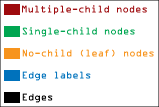 |
I will speak about different "generations" of suffix trees. It is my unofficial terminology, used only for this explanation. The "third generation suffix tree" is the true suffix tree. It takes up linear space, and it is what is built by Ukkonen's algorithm in linear time. The "second generation suffix tree" is a naive suffix tree which takes up quadratic space and hence is built in quadratic time. The "first generation suffix tree" is not really a suffix tree at all - it is a fairly dreadful and ugly quadratic-space, quadratic-time data structure. Its only advantage is that it is dead easy to construct by hand. Remember that while I use the different generations of suffix trees to explain the basic concepts, they are not actually built this way. Simply generating a first or second generation suffix tree takes quadratic-time, so if you want to generate a suffix tree in linear time, you must use Ukkonen's algorithm and can not do it via a first or second generation intermediate.
| Let us first work with the string DEADBEEF. We will make the first generation suffix tree for this string. We do this by listing all of the string's suffixes, making chains of nodes and edges for each suffix, and then attaching each chain to the root. Each edge is labeled with a symbol from the original string. The first symbols of a suffix appear on the edges closest to the root. In a first generation suffix tree, only the root has multiple children. Also, there is no real concept of the order of the children - I arbitrarily put the longest suffixes on the left, but this is only for illustration. It is a big mess. | 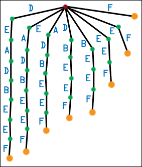 |
| We can make the messy first generation tree a little neater. Any time a node has multiple children edges labeled with the same symbol, combine those edges (and the nodes they lead to) into one. However, you must also preserve subtrees, so you may create multiple-children nodes in the process. Repeat until no nodes have multiple children edges labeled with the same symbol. This produces the second-generation suffix tree. Note that in the first generation suffix tree for DEADBEEF, the root has two D edges leading out from one. One edge leads to a node which has a B-E-E-F subchain, while the other edge leads to a node with a E-A-D-B-E-E-F subchain. When we combine these, the root ends up with a single D edge leading to a single node. That node, in turn, has two subchains as its children. The chains start with different symbols, so no further combination can be done here. For DEADBEEF, only a little combination has to be done, but in general, many multiple-children nodes can be created. Here, I have ordered the edges leading out of any node lexicographically - A edges appear to the left of B edges, and so forth. Second generation suffix trees have the property that each node can have at most Q children edges, where Q is the number of symbols in the alphabet, and no node can have multiple children edges labeled with the same symbol (otherwise, they would have been combined together). This is a fairly nice property. | 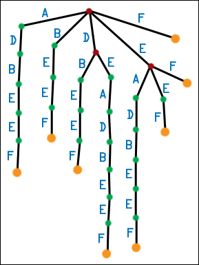 |
Suppose that we are given the [second generation] suffix tree for DEADBEEF. Never mind that it is quadratic-space, or that it took quadratic time to generate. We have the tree stored in memory. Note the following astounding ability we now have. Given ANY string of length M, we can determine whether it is a substring of DEADBEEF regardless of the length N of DEADBEEF. (We may as well have a suffix tree for the contents of the Library of Congress, instead of an 8-letter word for hamburger, and it would not affect the performance of this substring-matching algorithm at all, as long as we get the suffix tree already generated for us.) How do we do this? Suppose we want to know if ADB is a substring of DEADBEEF. Start at the root of the suffix tree. Look at the first symbol of ADB. Is there an edge labeled with that symbol? Yes, there is. Go to that node. Look at the next symbol (D). Is there an edge labeled with that symbol? Yes, there is. Go to that node. Look at the next symbol (B). Is there an edge labeled with that symbol? Yes, there is. Go to that node. Now we have exhausted the string we were given, so it is a substring of DEADBEEF. This took us O(M) time, and it did not matter how many symbols were in DEADBEEF itself (so it may as well have been the Library of Congress). If at any time we try to find an edge labeled with a symbol, and that edge doesn't exist, then we know the string we were given is not a substring. Compare this to any naive algorithm you can think of for substring matching, and it will certainly be worse than O(M) - it will have N in there, somewhere. Also note that, once you have generated a suffix tree for a string, you can do as many substring-matching problems as you like, and you just keep the tree constant in memory, walking through it. Suffix tree generation is a one-time cost. This is very useful in the field of genetics - you can search through the human genome itself, just by walking through a suffix tree!
However, second generation suffix trees are quadratic-space, though not as bad as first generation suffix trees, and hence take quadratic time to generate. We can do better!
| This is a third generation (for real this time) suffix tree. We relax the requirement that edges are labeled by single symbols of the original string. Instead, edges are labeled by substrings of the original string. We "path compress" the second generation suffix tree, and remove all single-children nodes. A [real] suffix tree has only multiple-children nodes and leaf nodes, never single-children nodes. We can still use the substring-matching algorithm with a real suffix tree, though we might not leap to a new node after looking at every symbol. It can be proven that the number of nodes in a real suffix tree is linear in the number of symbols of the original string. What may [should!] concern you is the space required to store the labels for the edges! After all, that's a lot of symbols. Luckily, any given edge can be stored in constant space. Instead of storing the symbols themselves, we store indices into the original string. We only need two, and we can define any substrings we like. This is a linear-space suffix tree, just as useful (more useful!) than a second generation suffix tree, and we can use it for substring matching or Burrows-Wheeler sorting. How can we use it for Burrows-Wheeler sorting? Look at the leaf nodes of the suffix tree for DEADBEEF. They exactly correspond to the suffixes of DEADBEEF. Furthermore, by doing a simple depth-first search (visiting edges with lexicographically lesser first symbols before edges with lexicographically greater first symbols), we will hit the leaf nodes/suffixes in lexicographic order! So, if we build this linear-space suffix tree in linear time (with Ukkonen's algorithm) and then do a depth-first search (also linear time), we will have sorted the suffixes of the string, which is exactly what the Burrows-Wheeler Transformation needs! | 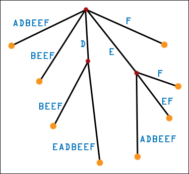 |
| Well, not quite. There is a problem, and if you paid attention to the Circular Shifts = Suffixes section, you may be catching on. What happens when one suffix is the prefix of another suffix? Here is the first generation suffix tree for MOOMOO. | 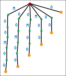 |
| And here is the second-generation suffix tree for MOOMOO. Uh oh, six suffixes and only three leaf nodes. | 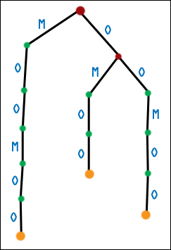 |
| The real suffix tree for MOOMOO also has three leaf nodes, of course. What has happened? If one suffix is the prefix of another suffix, then it will end midway through the tree, and it will not get a leaf node of its own. It may not even end on an internal node - it could end (conceptually) in the middle of an edge! While we can still do substring matching no problemo, we are in for some trouble if we expect the leaf nodes to exactly correspond to suffixes. | 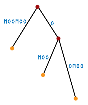 |
| The solution, as before, is to add a sentinel character. Not only does a sentinel character make sorting the suffixes of the augmented string identical to sorting the circular shifts of the augmented string, but adding a sentinel character ensures that suffixes in a suffix tree correspond exactly to leaf nodes! This is the best of both worlds! Here is the first generation suffix tree for MOOMOO$. (Hopefully it is not necessary to see this; I include it for completeness). | 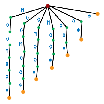 |
| Here is the second generation suffix tree for MOOMOO$. | 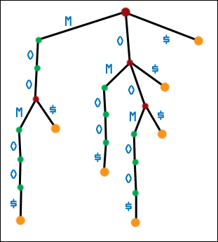 |
| And here is the real, path-compressed, third generation suffix tree for MOOMOO$. Note: seven suffixes, seven leaf nodes. (I have defined $ to be greater than all other symbols.) Depth-first traversal of this tree gives the suffixes of MOOMOO$ in sorted order. Note that DEADBEEF ended with F, which didn't appear anywhere else in the string. This fake sentinel hid the problems with making a suffix tree for a bare string. As before, always add a sentinel to a string before making a suffix tree for that string, if you want suffixes to correspond exactly with leaf nodes. It hurts nothing, even in the case of DEADBEEF. | 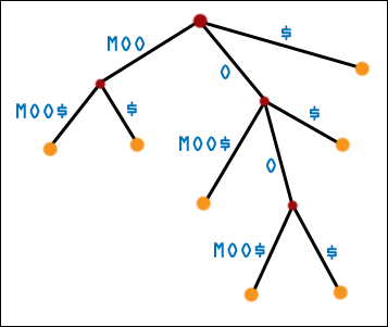 |
References
U. Manber and E. Myers, "Suffix Arrays: A New Method for On-Line String Searches", SIAM Journal on Computing 22, 5 (1993), 935-948. Available online.
M. Burrows and D. J. Wheeler, "A Block-Sorting Lossless Data Compression Algorithm", Digital Systems Research Center Research Report 124 (1994). Available online.
B. Balkenhol, S. Kurtz, Yu. M. Shtarkov, "Modifications of the Burrows and Wheeler Data Compression Algorithm", in DCC: Data Compression Conference, IEEE Computer Society TCC (1999). Available online.
B. Balkenhol, Yu. M. Shtarkov, "One Attempt of a Compression Algorithm Using the BWT", Preprint 99-133, SFB343: Discrete Structures in Mathematics, Faculty of Mathematics, University of Bielefeld (1999). Available online.
E. Ukkonen, "On-Line Construction Of Suffix Trees", Algorithmica (1995) 14: 249-260. All pages: ukkonen.tar (3.6 MB); Individual pages:
1
2
3
4
5
6
7
8
9
10
11
12
E. M. McCreight, "A Space-Economical Suffix Tree Construction Algorithm", Journal Of The Association For Computing Machinery, Vol. 23, No. 2, April 1976, pp. 262-272. All pages: mccreight.tar (4.1 MB); Individual pages:
1
2
3
4
5
6
7
8
9
10
11
Source Code
The bwtzip codebase is a toolbox of algorithms that work on STL vectors. In addition to bwtzip itself, there are functions which can compute SHA-1 or SHA-512 cryptographic hashes, can compress data using zlib or bzip2, can read and write files, and can work with PNG files.
A Makefile is included; typing make will print out a list of the applications which can be built. Each application corresponds to a main_appname.cc file, which is extremely short. The bwtzip code itself does the heavy lifting. One application, main, is a dummy: you can insert anything you like there to experiment with the algorithms. Alternative versions of bwtzip that use different algorithms for the BWT sort are provided.
Documentation
Currently, the entire bwtzip project is very sparsely documented. Look in the .hh files for explanations of the data structures and algorithms.
Known Issues
- An adaptive Huffman coder, using the same probability model as the current arithmetic coder, would be interesting to see. Unfortunately, a naive implementation of adaptive Huffman using the present routines proved to be extraordinarily inefficient. Joergen Ibsen's implemention of adaptive Huffman does not yet use the exact same probability model as the arithmetic coding routines.
- The suffix tree algorithm still consumes a large amount of memory, about 50 bytes per input byte. This can theoretically be reduced to 20. I would settle for 40.
- The suffix tree algorithm currently performs a lot of small allocations and deletions.
- bwtzip lacks the Bentley-Sedgewick and Larsson-Sadakane algorithms.
Corpuses
The contents of the corpuses are as follows.
Large English Text Corpus:
1dfre10.txt  - The History of The Decline and Fall of the Roman Empire, Volume 1 by Edward Gibbon
2000010a.txt - 20,000 Leagues Under the Sea by Jules Verne
2city12.txt  - A Tale of Two Cities by Charles Dickens
2dfre11.txt  - The History of The Decline and Fall of the Roman Empire, Volume 2 by Edward Gibbon
3dfre10.txt  - The History of The Decline and Fall of the Roman Empire, Volume 3 by Edward Gibbon
4dfre10.txt  - The History of The Decline and Fall of the Roman Empire, Volume 4 by Edward Gibbon
5dfre11.txt  - The History of The Decline and Fall of the Roman Empire, Volume 5 by Edward Gibbon
6dfre10.txt  - The History of The Decline and Fall of the Roman Empire, Volume 6 by Edward Gibbon
7crmp10.txt  - Crime and Punishment by Fyodor Dostoyevsky
blkhs10.txt  - Bleak House by Charles Dickens
cnmmm10.txt  - On the Economy of Machinery and Manufacture by Charles Babbage
cprfd10.txt  - David Copperfield by Charles Dickens
cwgen11.txt  - The Memoirs of Ulysses S. Grant, William T. Sherman, and Philip H. Sheridan
dosie10.txt  - Reflections on the Decline of Science in England by Charles Babbage
dscmn10.txt  - The Descent of Man by Charles Darwin
dyssy10b.txt - The Odyssey of Homer, translated by Alexander Pope
feder16.txt  - The Federalist Papers
flat10a.txt  - Flatland: A Romance of Many Dimensions by Edwin Abbott Abbott
grexp10.txt  - Great Expectations by Charles Dickens
grimm10a.txt - Household Tales by The Brothers Grimm
iliab10.txt  - The Iliad of Homer, translated by Lang, Leaf, and Myers
jargon.html  - The Jargon File 4.3.3
lnent10.txt  - The Entire Writings of Abraham Lincoln
lwmen10.txt  - Little Women by Louisa May Alcott
mtent13.txt  - The Entire Writings of Mark Twain
nkrnn11.txt  - Anna Karenina by Leo Tolstoy, translated by Constance Garnett
otoos610.txt - On the Origin of Species, 6th Edition, by Charles Darwin
pandp12.txt  - Pride and Prejudice by Jane Austen
pwprs10.txt  - The Pickwick Papers by Charles Dickens
sense11.txt  - Sense and Sensibility by Jane Austen
slstr10.txt  - Sidelights on Astronomy and Kindred Fields of Popular Science by Simon Newcomb
suall10.txt  - All State of the Union Addresses up to January 29, 2002
tmwht10.txt  - The Man Who Was Thursday by G. K. Chesterton
trabi10.txt  - Theodore Roosevelt, An Autobiography
twtp110.txt  - The Writings of Thomas Paine, Volume 1
twtp210.txt  - The Writings of Thomas Paine, Volume 2
vbgle11a.txt - A Naturalist's Voyage Round the World by Charles Darwin
warw11.txt   - The War of the Worlds by H. G. Wells
world02.txt  - The 2002 CIA World Factbook
wrnpc10.txt  - War and Peace by Leo Tolstoy
Large Source Code Corpus:
gcc-3.2.1.tar    - gcc 3.2.1 source code
linux-2.4.20.tar - Linux kernel 2.4.20 source code
Human Genome Corpus:
01hgp10a.txt - The Human Genome, Chromosome 1
02hgp10a.txt - The Human Genome, Chromosome 2
03hgp10a.txt - The Human Genome, Chromosome 3
04hgp10a.txt - The Human Genome, Chromosome 4
05hgp10a.txt - The Human Genome, Chromosome 5
06hgp10a.txt - The Human Genome, Chromosome 6
07hgp10a.txt - The Human Genome, Chromosome 7
08hgp10a.txt - The Human Genome, Chromosome 8
09hgp10a.txt - The Human Genome, Chromosome 9
0xhgp10a.txt - The Human Genome, Chromosome X
0yhgp10a.txt - The Human Genome, Chromosome Y
10hgp10a.txt - The Human Genome, Chromosome 10
11hgp10a.txt - The Human Genome, Chromosome 11
12hgp10a.txt - The Human Genome, Chromosome 12
13hgp10a.txt - The Human Genome, Chromosome 13
14hgp10a.txt - The Human Genome, Chromosome 14
15hgp10a.txt - The Human Genome, Chromosome 15
16hgp10a.txt - The Human Genome, Chromosome 16
17hgp10a.txt - The Human Genome, Chromosome 17
18hgp10a.txt - The Human Genome, Chromosome 18
19hgp10a.txt - The Human Genome, Chromosome 19
20hgp10a.txt - The Human Genome, Chromosome 20
21hgp10a.txt - The Human Genome, Chromosome 21
22hgp10a.txt - The Human Genome, Chromosome 22
https://nuwen.net/bwtzip.html (updated 2/13/2006)
Stephan T. Lavavej
Home: stl@nuwen.net
Work: stl@microsoft.com
This is my personal website. I work for Microsoft, but I don't speak for them.